Urban Geocomputation:
Two Studies on Urban Form and Its Role in Altering Climate
Jackson Voelkel
November 28, 2017
A thesis submitted in partial fulfillment of the
requirements for the degree of
Master of Urban Studies
Thesis Committee:
Vivek Shandas, Chair
Liming Wang
David S Banis
Portland State University 2018
Introduction
Warming Climate, Growing Cities
Geocomputation
- Disabling Technology: Oversimplification by standardization
- Enabling Technology: The right tools at the right time
“… a conscious attempt to move the research agenda back to geographical analysis and modelling.”
“… not compromising the geography, nor enforcing the use of unhelpful or simplistic representations.”
“… a conscious effort to explore […] the doubly-informed perspective of geography and computer science.”
Gahegan, Mark. “GeoComputation,” 2017. http://www.geocomputation.org/what.html.
Structure of Thesis
- Two chapters
- Seperate Analyses
Chapter 1
- Urban form
- Microclimates
- Residential energy consumption
- Climate change
Chapter 2
- Urban trees (a factor in form)
- Tree types
- Urban Heat Island Effect
- NO\(_2\)
Urban Form and Residential Energy Expenditures: A Potential for Climate Change Intervention
Introduction
Urban Populations
- Currently, majority of humans reside in cities
- 2.5 billion more people in cities by 2050
Climate Change
- Temperature increases
- Changes to:
- Agriculture
- Forestation Levels
- Sea Levels
- Ecosystems
- Human Health
- Energy Consumption
Urban Sustainability
- Green Infrastructure
- Tree plantings
- Urban Heat
- Storm water
- Air Pollution
Urban Form, Energy Consumption, and Climate Change
Ko, 2013
- Urban areas use the most energy
- Between 67% and 76% of energy consumption
- Cities must use more energy due to climate change
- Urban form influences energy consumption
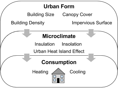 Urban form and its effect on residential energy consumption. Adapted from Ko (2013).
Akbari, 2002
- Vegetation and tree configuration may reduce energy use
- … reduced energy production
- … reduced emissions
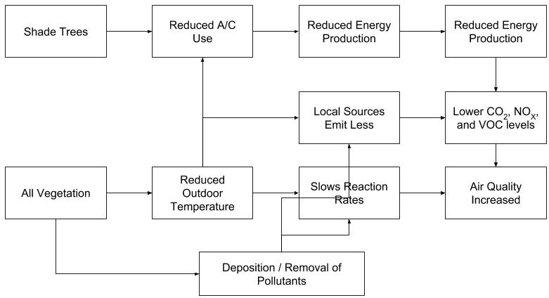 Urban vegetation and its effect on detrimental aerosols. Adapted from Akbari (2002).
Incomplete Framework
- Decreased emissions = mitigation of climate change
- Feedback loop
- Lower global temperatures lead to lower local temperatures
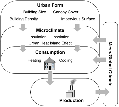 Urban form’s effect on micro/global climate change and the positive feedback loop therein.
Existing Studies
- Usually fit into three paradigms
Type 1: Generalized / Global
- City vs. city analysis
- Assumes uniformity in spatial distribution of urban features
- e.g. trees
Common software/models: URBMET, DOE-2.1C
Type 2: Detailed / Semi-Localized
- Requires exact metrics of trees
- e.g. specific species, diameter at breast height
- Eventually generalizes to larger geometries
- e.g. U.S. Census enumeration units
Common software/models: iTree, CITYgreen
Type 3: Precise / Localized
- Intra-building analysis
- Requires detailed knowledge of building construction materials
- Limited to a handful of buildings, often a single buildings
Common software/models: ENVI-met, EnergyPlus
Needed: A Hybrid Method
This must:
- be conducted at a city- or regional-scale
- include highly-resolved descriptions of landforms
- leverage a large sample size of building energy use observations
- account for variations in building stock (e.g. size, vintage)
Hypotheses
Hypothesis 1: residents located in areas of higher temperatures (driven by complex measures of urban form) experience an additional burden in terms of energy expenditures.
Hypothesis: the configuration of canopy around a residential building (at multiple distances and directions) reduces annual energy expenditures.
Methods
Study Area
Portland Metropolitan Area (PMA)
- 24 cities/towns
- ~1.46 Million residents
- 1218km\(^2\)
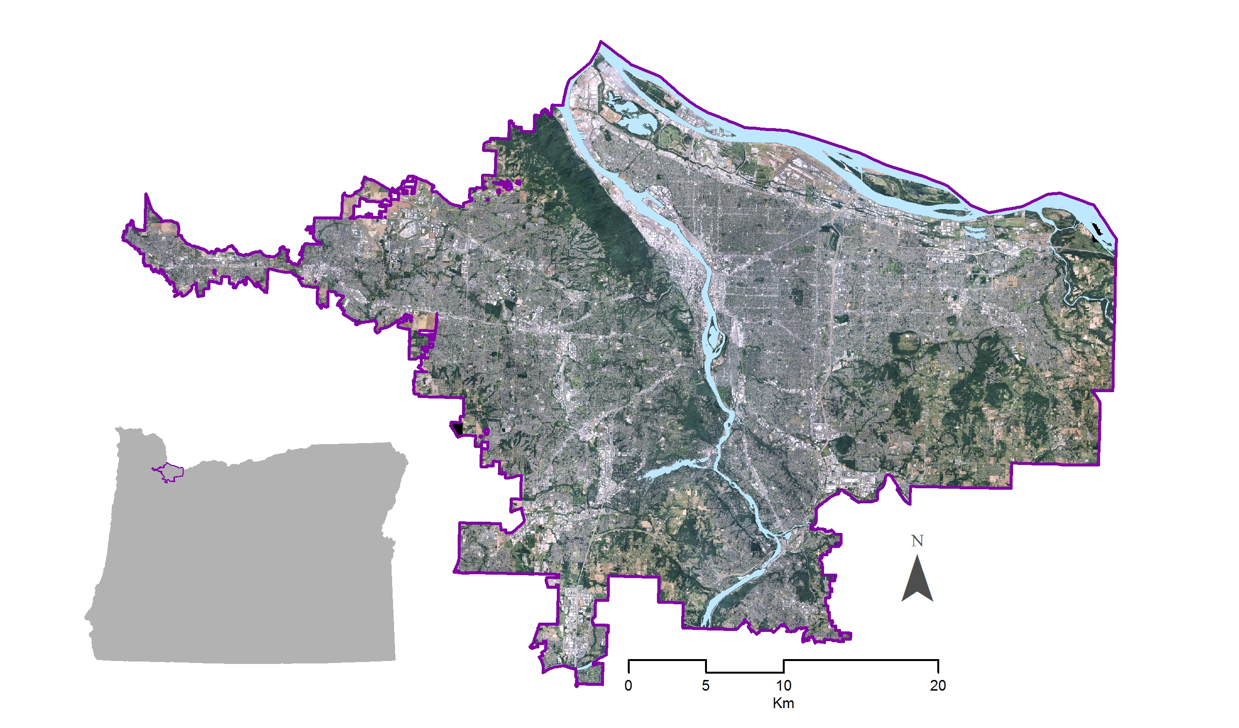 Aerial Imagery of the PMA.
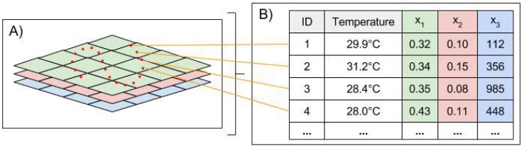
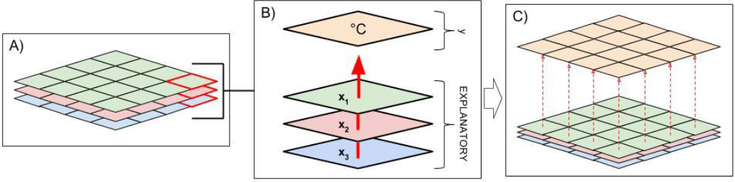
Data
Energy Consumption
- Obtained through Energy Trust of Oregon
- sub-building (i.e. per unit) measure of electricity and natural gas consumption
- yearly total
- Required extensive cleaning and geocoding for spatial analysis
- conducted by Tim Hitchins and Alec Trusty, SUPR Lab, PSU
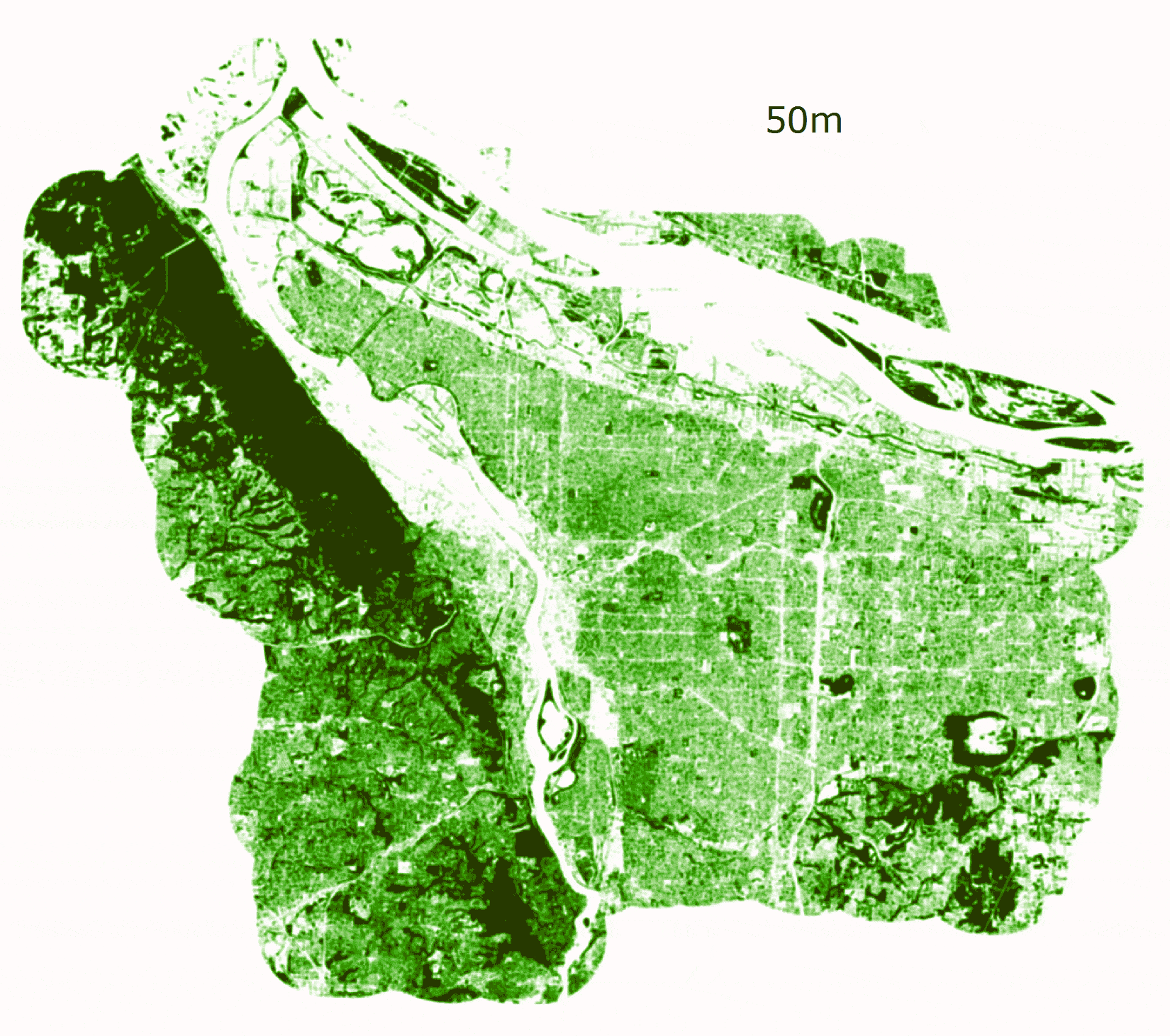
Canopy Cover
- Provided by Oregon Metro’s Regional Land Information System (RLIS)
- 1m\(^2\) resolution over the entire region
- 2014 LiDAR and Infrared Imagery
- Represents Canopy Height
Conversion to binary canopy representation
\(RO = (RC_i > 0 → RO_i = 1) ∧ (¬RC_i= NULL → RO_i = 0)\)
RC = Input canopy data
RO = Output canopy data
i = Individual raster pixel
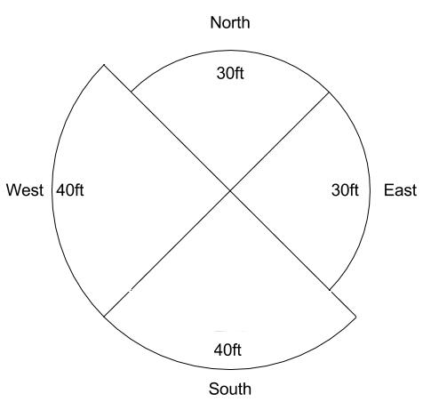
Multi-distance multi-directional canopy configuration assessment
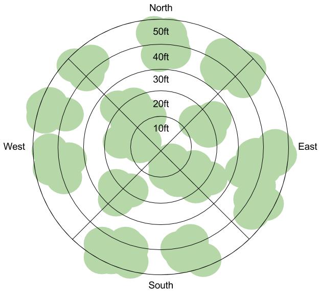
Directional Canopy Assessment.
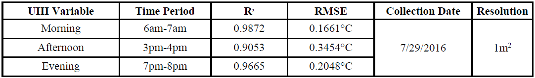
Urban Heat
- Adapted from Voelkel and Shandas (2017)
- Include information for the entire region
- As a measure of form!
- modeled from complex relations of urban form (more in chapter 2)
Unit of Analysis
kWh and thm converted to total expenditure
- Building-level assignment of attributes:
- buildings
- tax lots
- tree configuration (both cover and volume)
- urban heat
- energy expenditure
- number of energy meters per building
Regression
Ordinary Least Squares (OLS)
- Many Assumptions
- homoscedasticity
- limited multicollinearity in independent variables
- Often the best linear unbiased estimator of a dependent variable
Tobit Regression
- “Censored” model
- Potentially increases performance by simulating more realistic outcomes
- Overall, quite similar to OLS
Model Selection
- Root Mean Square Error (RMSE)
- Akike Information Criterion (AIC)
Spatial Autocorrelation
- Where observations are situated in space alters the observed values
- Violates assumption of independence
- Assess Moran’s I with a Monte Carlo simulation
Results
Model Selection
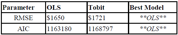
OLS is the preferred model based on both RMSE and AIC!
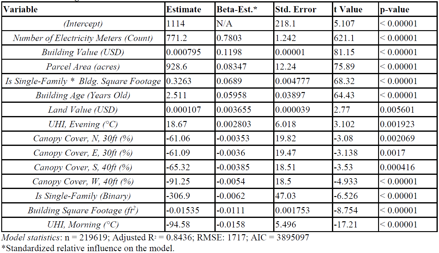
OLS
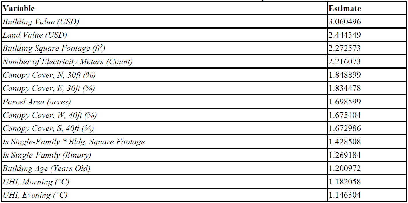
The final model specification includes 14 variables:
- Number of Electricity Meters (Count)
- Building Value (USD)
- Parcel Area (acres)
- Is Single-Family * Bldg. Square Footage
- Building Age (Years Old)
- Land Value (USD)
- UHI, Evening (°C)
- Canopy Cover, N, 30ft (%)
- Canopy Cover, E, 30ft (%)
- Canopy Cover, S, 40ft (%)
- Canopy Cover, W, 40ft (%)
- Is Single-Family (Binary)
- Building Square Footage (ft\(^2\))
- UHI, Morning (°C)
OLS Estimates
OLS Multicollinearity
Spatial Autocorrelation
- I = 0.0305
- p-value = significant
Though significant, the actual degree of clustering is minimal!
Discussion
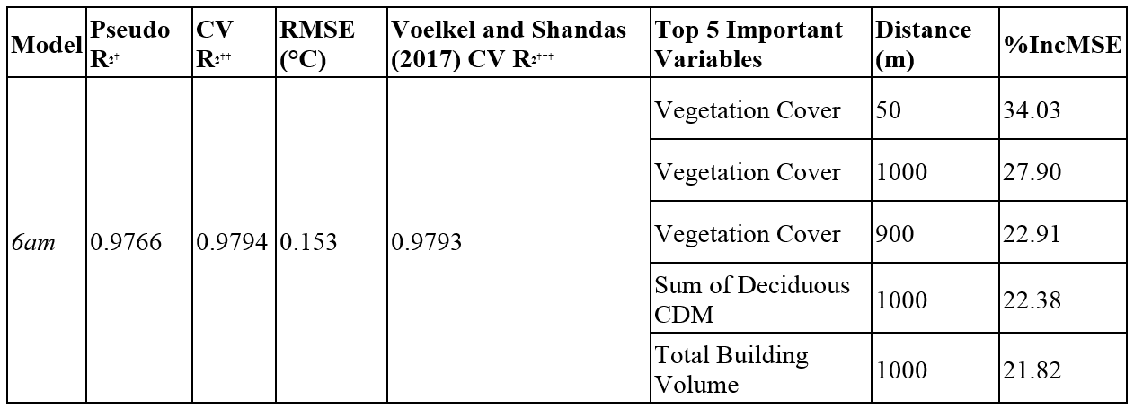
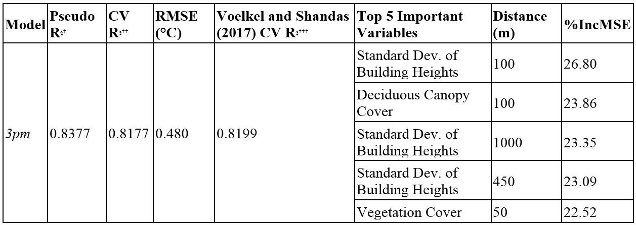
Urban Heat
- Afternoon UHI
- Dropped (insignificant)
- Lowest performance of UHI models
- Less energy consumption between 3pm and 4pm
Morning vs. Evening
- Opposite effects
- Morning: +1°C = -$94.58/year
- Evening: +1°C = +$18.65/year
- Morning temperatures hardly fluctuate
- Evening temperatures are far hotter
- Vulnerability
- Actual burden
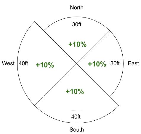
Canopy Configuration
- Canopy volume configuration
- insignificant
- Canopy cover configuration
- similar to literature…
- … except to the North!
30ft-40ft in all directions = reduction in energy expenditure
- Effects beyond property lines
Patterns in Outlier Observations
- Regression diagnostics
- Identification of 12 Observations
- Retirement homes (many units, few energy meters)
- Detox Clinics (medical equipment)
- Misclassifications (issues in RLIS data)
- Removal results in 8.74% increase in expenditure variation explanation
Applications of results
- Measure urban form alterations
- Tree removals
- Targeted tree plantings
Increasing Canopy Cover
- 1 home: $27.87/year
- 300 homes: $8,361.60/year
- 1980 homes: $55,186.56/year
- 465,368 homes: $12,970,737/year
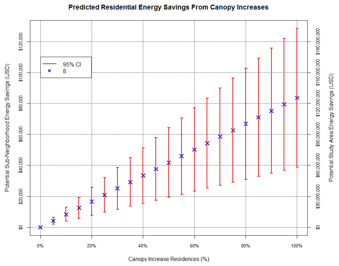
- Web map application?
Temporal Resolution
- Literature is often monthly
- UHI is a snapshot
- representative of form (significantly impacts yearly expenditure)
Conclusion
UHI as an indicator for energy consumption
Hypothesis: residents located in areas of higher temperatures (driven by complex measures of urban form) experience an additional burden in terms of energy expenditures.
Likely!
Canopy configuration as mitigator of energy consumption
Hypothesis: the configuration of canopy around a residential building (at multiple distances and directions) reduces annual energy expenditures.
Likely!
Urban Form as an Intervention
- Increase trees, reduce UHI-prone landscapes
- Microclimates present lowered temperatures
- Energy consumption is reduced
- Energy production is reduced
- Global temperature increase rate drops
- Less global effects (heating) on microclimates
- etc.
The Role of Broad Tree Functional Types in Urban Heat Island and Nitrogen Dioxide Exposure Models
Introduction
Cities versus Nature
- Mid 19th to early 20th Century
- Often a dichotomous relationship
- Georg Simmel
- Urban = Absence of nature
- Louis Wirth
- Urban = “removal of the organic”
- Frederick Law Olmstead
- Impossible to integrate
- No interaction
- Parks as pure nature within the city
- Georg Simmel
Cities with Nature
- Nature and cities aren’t mutually-exclusive
- Urban nature: street trees, open spaces
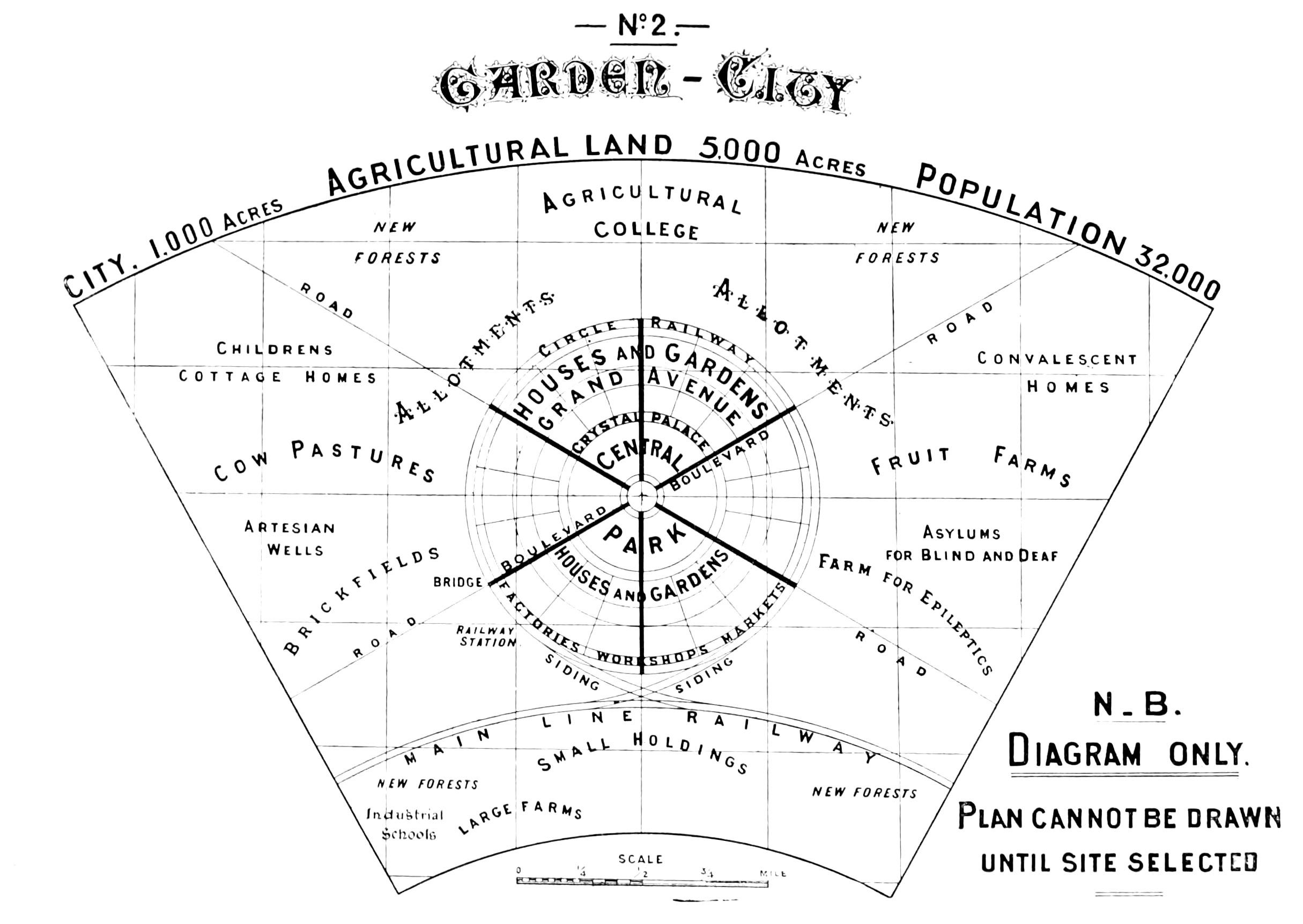
- Ebenezer Howard
- “Garden Cities”
Trees and Exposure
Roger S. Ulrich “View through a Window May Influence Recovery from Surgery.” (1984)
- Trees decrease healing times
Trees and Exposure
- Reduced number of ‘small for gestational age’ births
- Reduced air pollution
- Cooling of cities
- reduced risk of heat-realted illnesses
Tree functional types
- “tree” effects are known
- but what types?
- How do these broad tree functional types (BTFT) play out in different exposure scenarios?
- UHI vs air pollution
Hypothesis 1:
Evergreen trees have a greater effect on temperatures than deciduous.
- Denser
- potentially trap more cool air
Hypothesis 2:
Evergreens will reduce NO\(_2\) more than deciduous.
- Structure
- ‘brush-like’
Methods
Study Area
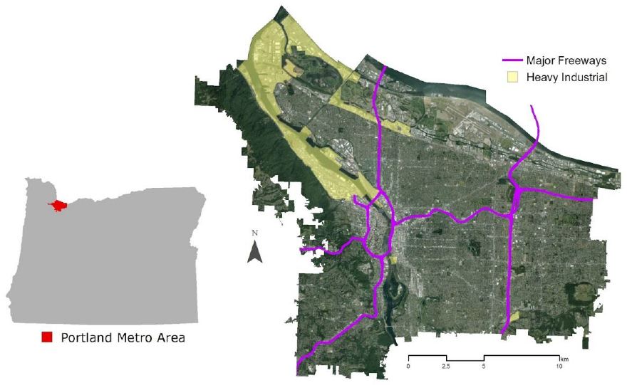
Data
Land Use / Land Cover
- LiDAR- and orthoimagery-derived
- high-resolution laser scanning system
- infrared imagery
- Buildings
- Mean height
- Volume
- Standard Deviation of heights
- Low-laying vegetation (under 10ft)
- Tree canopy
- laser-penetrability-adjusted crown volume (3D)
- ground cover (2D)
Broad Tree Functional Type (BTFT)
1m\(^2\) resolution; 88% Overall Accuracy; \(\kappa\) = ~0.75
Urban Heat and Air Pollution Measurements and Models
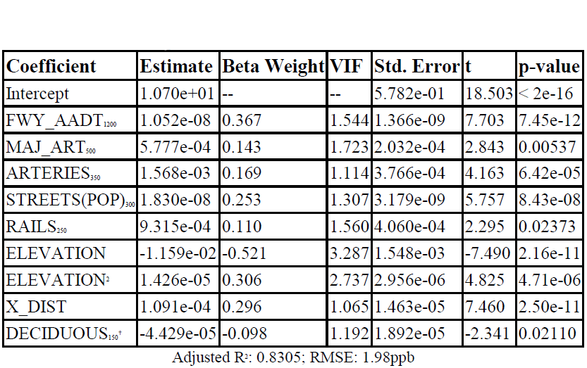
Rao et al. (2014) - NO2 Model
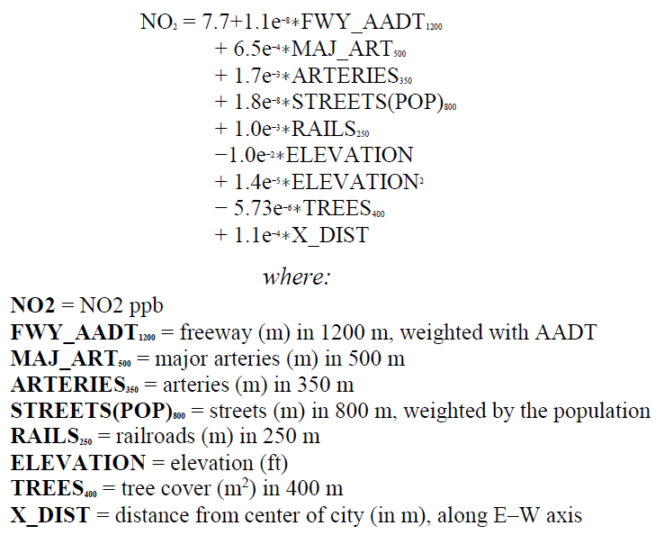 R\(^2\) = 0.80; RMSE = 2.2ppb
Continuous Surface Land Use / Cover Regression (CS-LUR)
Continuous Surface Land Use / Cover Regression (CS-LUR)
- Multi-distance land use descriptions
- ‘Buffers’
- Can decrease spatial autocorrelation
Urban Heat Island Effect Modeling
Surface Prediction
BTFT Variable Effect
- Model is specified and surface is predicted
- Original model is fed into new data cube
- Variable of interest set to 0
- Difference is measured between original predicted surface and ‘zeroed’ surface is calculated
This new raster represents the variable’s effect.
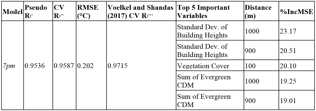
Calculated the effect of evergreen vs. deciduous for morning, afternoon, and evening
Mobile-source Air Pollution Modeling
- Test significance of BTFT variables as replacements for plain “canopy”
- Rao et al. (2014): 144 sites
- 88 within the City of Portland
Results
Urban Heat Island Effect CS-LUR
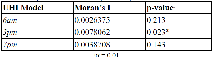
Spatial Autocorrelation of UHI Model Error
BTFT Variable Effect
- 6 rasters = 5,022,000,000 pixels
- 1 million pixel sample
- t-test: Deciduous Effect vs. Evergreen Effect
- Evergreen trees reduce temperatures more at all times
Mobile-source Air Pollution Modeling
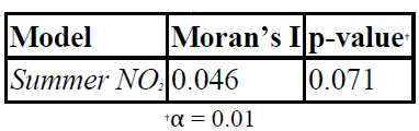
Spatial Autocorrelation of NO2 Model Error
Discussion
BTFT and the Urban Heat Island Effect
Hypothesis: BTFT will increase UHI model performance
Likely!
- Pruning
- Similar results…
- … half the number of CARTs
- Reduced chance of over-fitting
Hypothesis: evergreen trees have a greater effect on temperatures than deciduous
Likely!
- Evergreen share of total trees:
- Cover: 35.55%
- Volume: 43.48%
- Fewer trees doing more!
Reflection: Using CS-LUR
Pros
- High predictive accuracy
- Low Spatial Autocorrelation
- Based in fundamentals of LUR
- No need for additional interpolation
- Error introduction
Cons
- Computationally expensive
- Many days to run a single prediction
- … using 16 cores with 757GB of RAM limit
- Large data sizes
- Datacube: 2.056TB
- Output Surfaces: 20GB each
- Low explanatory power
- No coefficients
BTFT and Mobile-Source Air Pollution
Hypothesis: Evergreens will reduce NO\(_2\) more than deciduous.
Unlikely!
- Deciduous within 150m
- Only significant variable
- Variation of NO\(_2\) explained increases by ~ 3%
- RMSE reduced by 0.22ppb
- Minimal reductions
Rao et al. (2014) - canopy influence
1m\(^2\) increase of deciduous canopy cover within 400m: Reduction of 0.00000573ppb
Current study - canopy influence
1m\(^2\) increase of deciduous canopy cover within 150m: Reduction of 0.00004429ppb
Conclusion
Policy implications
Recommendation #1
In areas of increased air pollution, the planting of deciduous trees should be prioritized.
- along freeways
- near train yards
- near ports
Recommendation #2
In areas with pronounced urban heat islands, the planting of evergreen trees should be prioritized.