Spatial Regression I
GEOG 4/597: Advanced Spatial Quantitative Analysis, Winter 2021
Jackson Voelkel | Portland State University
Overview
- Regression in R
- Spatial Autocorrelation and Regression
- Spatial Regression
Regression
Ordinary Least Square (OLS)
- Line of best fit
(some) OLS Assumptions
- Normal distribution: Dependent Variable
- Robust
- Minimal multicollinearity
- Independence of observations
Running OLS in R
##
## Call:
## lm(formula = mpg ~ hp, data = mtcars)
##
## Residuals:
##     Min      1Q  Median      3Q     Max
## -5.7121 -2.1122 -0.8854  1.5819  8.2360
##
## Coefficients:
##             Estimate Std. Error t value Pr(>|t|)
## (Intercept) 30.09886    1.63392  18.421  < 2e-16 ***
## hp          -0.06823    0.01012  -6.742 1.79e-07 ***
## ---
## Signif. codes:  0 '***' 0.001 '**' 0.01 '*' 0.05 '.' 0.1 ' ' 1
##
## Residual standard error: 3.863 on 30 degrees of freedom
## Multiple R-squared:  0.6024, Adjusted R-squared:  0.5892
## F-statistic: 45.46 on 1 and 30 DF,  p-value: 1.788e-07
Visualizing OLS Fit
require(ggplot2)
mtcars %>% ggplot(aes(x=hp,y=mpg)) +
  geom_point(color='royalblue', size=2) +
  geom_smooth(
      formula = 'y ~ x',
      method = 'lm',
      color="red",
      size=0.5,
      se=F) +
  xlab("Horsepower") +
  ylab("Miles per Gallon") +
  ggtitle("Miles per Gallon vs. Horsepower")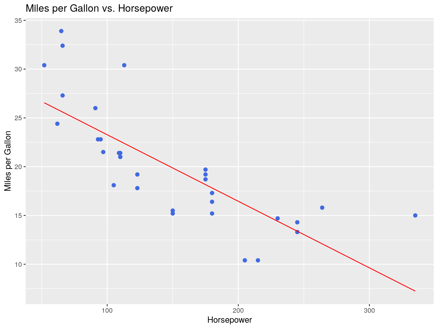
Our regression line is represented in red.
Assessing Fit: Residuals
mtcars %>% ggplot(aes(x=hp,y=mpg)) +
  geom_point(aes(color='Actual Values'), size=2) +
  geom_smooth(
      formula = 'y ~ x',
      method = 'lm',
      color="grey30",
      size=0.5,
      se=F) +
  geom_segment(
    aes(xend=hp, yend=mod$fitted.values,col='Residuals'),
    size=0.2) +
  # theme_minimal() +
  scale_color_manual("",values = c('royalblue','red')) +
  xlab("Horsepower") +
  ylab("Miles per Gallon") +
  ggtitle("Fitted (Modeled) Values and Residuals")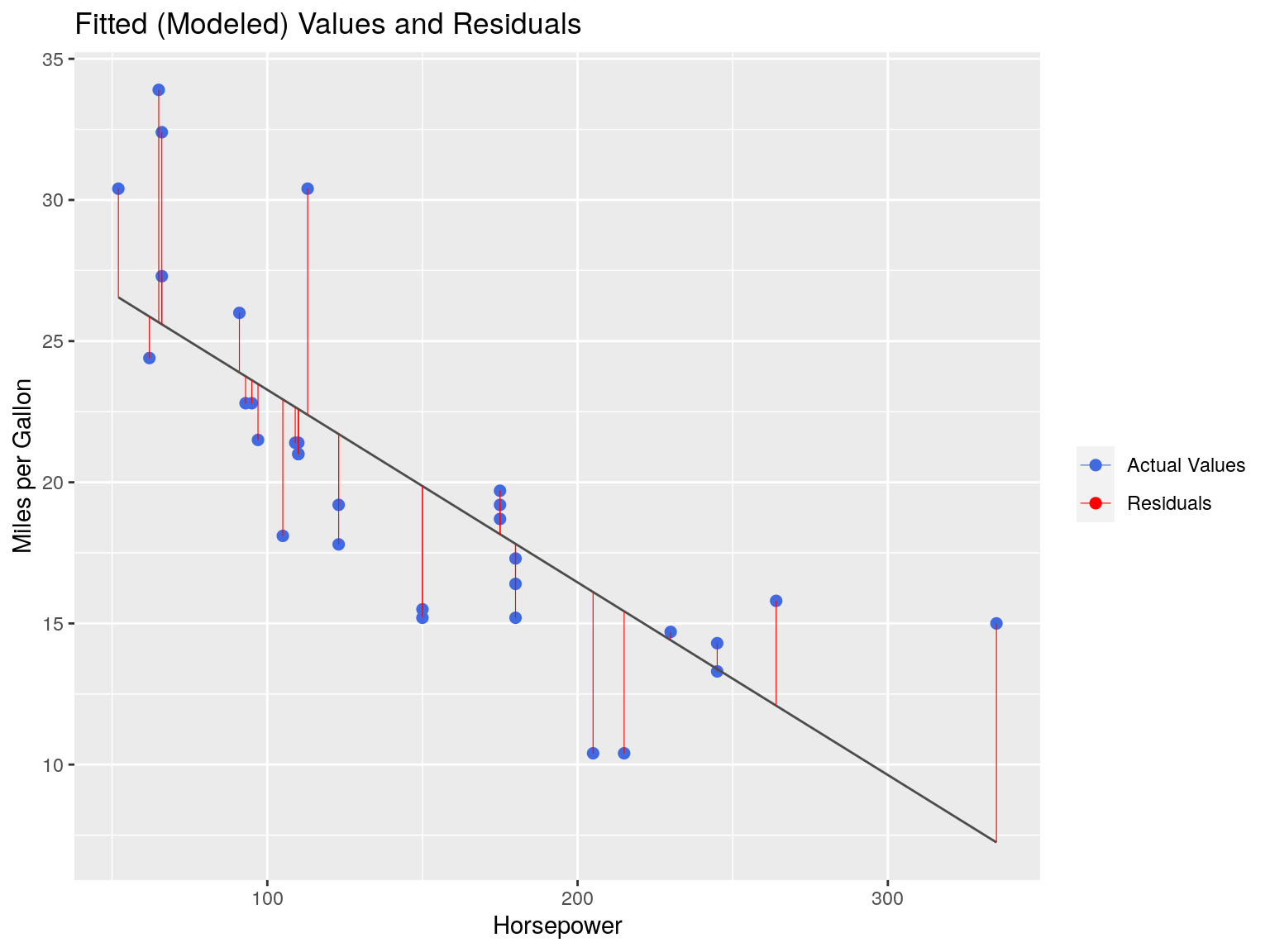
We can measure the ‘fit’ of our model by assessing the residuals.
OLS works by minimizing the Sum of Square Residuals (\(SS_R\))
\[SS_R = \sum\limits_{i=1}^{n}(y_i-\hat{y_i})^2\]
Residuals Tell a Story
The highest residual is 8.2360, for the Toyota Corolla:
##    Min. 1st Qu.  Median    Mean 3rd Qu.    Max.
## -5.7121 -2.1122 -0.8854 0.0000 1.5819 8.2360## mpg cyl disp hp drat wt qsec vs am gear carb
## Toyota Corolla 33.9 4 71.1 65 4.22 1.835 19.9 1 1 4 1The predicted value - based on our model - says that our mpg should be 25.66402 This is 8.2360 below the observed value.
##        1
## 25.66402
High residuals indicate that our model underpredicts.
The lowest residual is -5.7121, for the Cadillac Fleetwood:
##    Min. 1st Qu.  Median    Mean 3rd Qu.    Max.
## -5.7121 -2.1122 -0.8854 0.0000 1.5819 8.2360## mpg cyl disp hp drat wt qsec vs am gear carb
## Cadillac Fleetwood 10.4 8 472 205 2.93 5.25 17.98 0 0 3 4The predicted value - based on our model - says that our mpg should be 16.11206. This is 5.7121 above the observed value.
##        1
## 16.11206
Low residuals indicate that our model overpredicts!
Residuals are expected, as the goal of OLS is to reduce the total residuals in the model, not necessarily create the ‘best predictor’
Accounting for More Variables
- We need to account for other variables
- Important variables like weight are not being factored in
Accounting for More Variables
##
## Call:
## lm(formula = mpg ~ hp + wt, data = mtcars)
##
## Residuals:
##    Min     1Q Median     3Q    Max
## -3.941 -1.600 -0.182  1.050  5.854
##
## Coefficients:
##             Estimate Std. Error t value Pr(>|t|)
## (Intercept) 37.22727    1.59879  23.285  < 2e-16 ***
## hp          -0.03177    0.00903  -3.519  0.00145 **
## wt          -3.87783    0.63273  -6.129 1.12e-06 ***
## ---
## Signif. codes:  0 '***' 0.001 '**' 0.01 '*' 0.05 '.' 0.1 ' ' 1
##
## Residual standard error: 2.593 on 29 degrees of freedom
## Multiple R-squared:  0.8268, Adjusted R-squared:  0.8148
## F-statistic: 69.21 on 2 and 29 DF,  p-value: 9.109e-12
Considerations
Should we always transform our data to a normal distribution?
- You were probably told yes, but this is a misconception!
How do we select independent variables?
- Use our logic!
- Do NOT just throw everything at it. Variable selection is itself a hypothesis.
Considerations
Multicolinearity:
##       hp       wt
## 1.766625 1.766625
Our independent variables must be exactly that: independent of one another!
Variance Inflation Factor (VIF)
##
## Call:
## lm(formula = mpg ~ ., data = mtcars)
##
## Residuals:
##     Min      1Q  Median      3Q     Max
## -3.4506 -1.6044 -0.1196  1.2193  4.6271
##
## Coefficients:
##             Estimate Std. Error t value Pr(>|t|)
## (Intercept) 12.30337   18.71788   0.657   0.5181
## cyl         -0.11144    1.04502  -0.107   0.9161
## disp         0.01334    0.01786   0.747   0.4635
## hp          -0.02148    0.02177  -0.987   0.3350
## drat         0.78711    1.63537   0.481   0.6353
## wt          -3.71530    1.89441  -1.961   0.0633 .
## qsec         0.82104    0.73084   1.123   0.2739
## vs           0.31776    2.10451   0.151   0.8814
## am           2.52023    2.05665   1.225   0.2340
## gear         0.65541    1.49326   0.439   0.6652
## carb        -0.19942    0.82875  -0.241   0.8122
## ---
## Signif. codes:  0 '***' 0.001 '**' 0.01 '*' 0.05 '.' 0.1 ' ' 1
##
## Residual standard error: 2.65 on 21 degrees of freedom
## Multiple R-squared:  0.869,  Adjusted R-squared:  0.8066
## F-statistic: 13.93 on 10 and 21 DF,  p-value: 3.793e-07
Great \(R^2\), but none of our independent variables are significant!
Variance Inflation Factor (VIF)
##       cyl      disp        hp      drat        wt      qsec        vs        am
## 15.373833 21.620241  9.832037  3.374620 15.164887  7.527958  4.965873  4.648487
##      gear      carb
##  5.357452  7.908747
Rule of thumb: under 10 for liberal, under 5 for conservative, under 4 for strict.
OLS and Spatial Data
An example
We will create a model predicting Median Household income as a function of Educational Attainment (% of the population 25+ with a bachelors degree or higher) and average household size in the Portland Metro Area.
Step 1: Getting the Data
suppressPackageStartupMessages(require(sf))
suppressPackageStartupMessages(require(tidycensus))
suppressPackageStartupMessages(require(tmap))
suppressMessages(tmap_mode('plot'))
cbg <- get_acs(
  geography = 'block group',
  state = "OR",
  county = c("Multnomah","Clackamas","Washington"),
  variables = c('B99121_001','B99152_001','B19013_001','B25010_001'),
  output = 'wide',
  geometry = TRUE) %>%
  mutate(
    edu = B99152_001E/B99121_001E,
    mhi = B19013_001E,
    hhs = B25010_001E
)tm_shape(cbg) +
tm_polygons(
col = 'mhi',
lwd = 0.2,
border.col = 'grey80',
title = "Median Household Income",
palette = 'Greens',
style = 'jenks') +
tm_layout(main.title = 'Portland Metro Area: Income Distribution')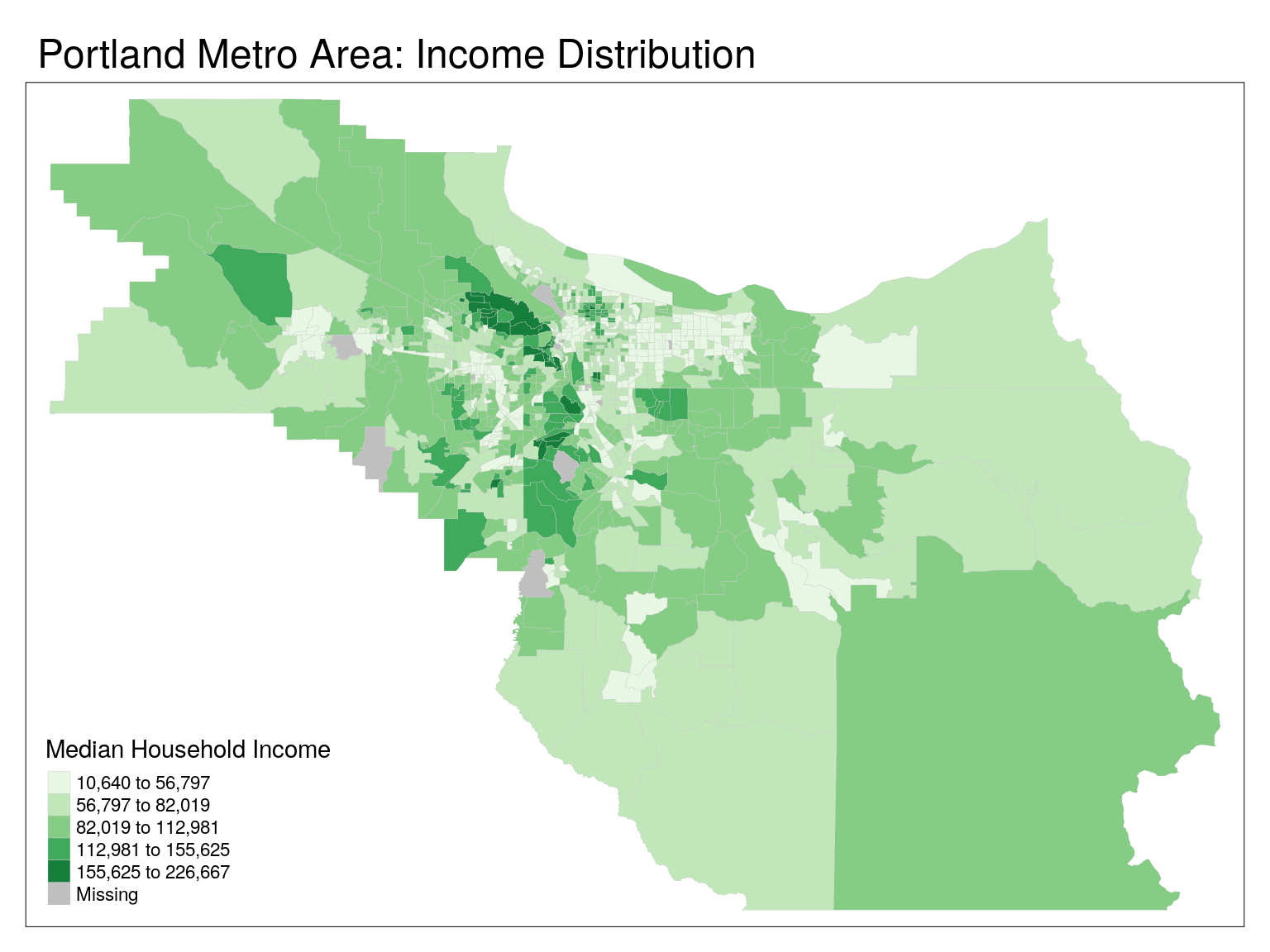
tm_shape(cbg) +
  tm_polygons(
    col = 'edu',
    lwd = 0.2,
    border.col = 'grey80',
    title = "Share of Adults 25+ with at \nLeast a Bachelors Degree",
    palette = 'Blues',
    style = 'jenks') +
  tm_layout(main.title = 'Portland Metro Area: Educational Attainment')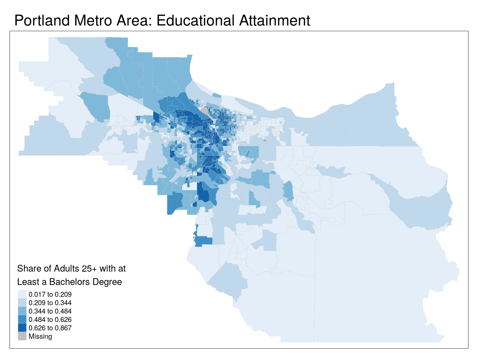
tm_shape(cbg) +
  tm_polygons(
    col = 'hhs',
    lwd = 0.2,
    border.col = 'grey80',
    title = "Average People per Household",
    palette = 'Oranges',
    style = 'jenks') +
  tm_layout(main.title = 'Portland Metro Area: Household Size')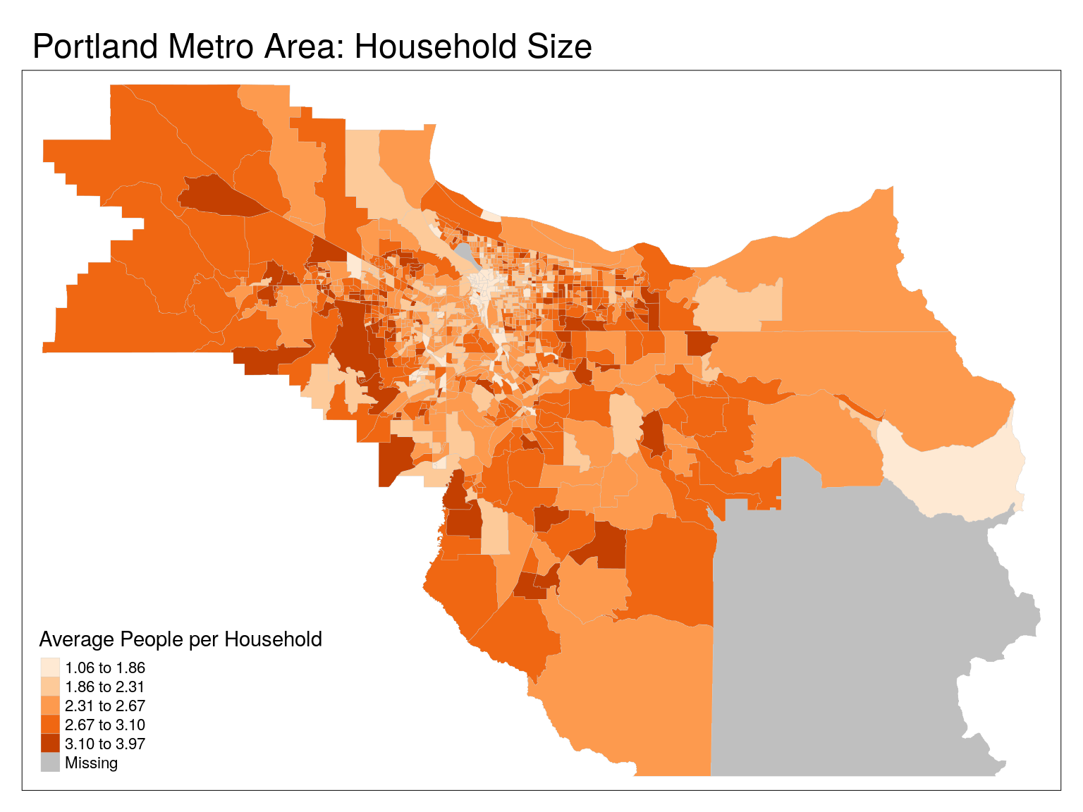
OLS Model
##
## Call:
## lm(formula = mhi ~ edu + hhs, data = cbg)
##
## Residuals:
##    Min     1Q Median     3Q    Max
## -59439 -13112   -165  12403  84948
##
## Coefficients:
##             Estimate Std. Error t value Pr(>|t|)
## (Intercept)   -62005       4318  -14.36   <2e-16 ***
## edu           132531       3514   37.71   <2e-16 ***
## hhs            35265       1433   24.60   <2e-16 ***
## ---
## Signif. codes:  0 '***' 0.001 '**' 0.01 '*' 0.05 '.' 0.1 ' ' 1
##
## Residual standard error: 20330 on 1025 degrees of freedom
##   (13 observations deleted due to missingness)
## Multiple R-squared:  0.6085, Adjusted R-squared:  0.6078
## F-statistic: 796.6 on 2 and 1025 DF, p-value: < 2.2e-16## edu hhs
## 1.117701 1.117701Multicollinearity is under control!
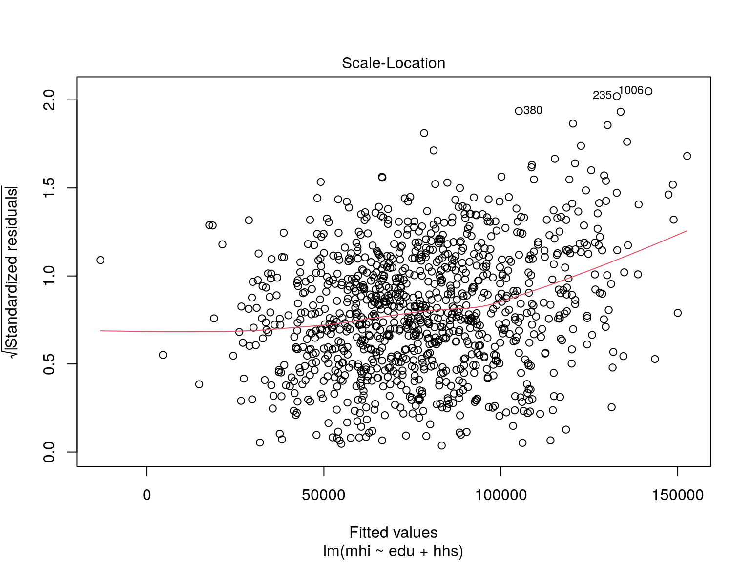
Our residuals don’t appear to have any strong pattern to them!
Same plot, with ggplot2:
data.frame(
residuals = mod$residuals^2 %>% sqrt(),
fitted = mod$fitted.values
) %>% ggplot(aes(x=fitted,y=residuals)) +
geom_point() +
xlab("Fitted Values") +
ylab("Standardized Residuals") +
geom_smooth(
method = 'gam',
col='red',se = FALSE) +
ggtitle("Residuals vs. Fitted Values")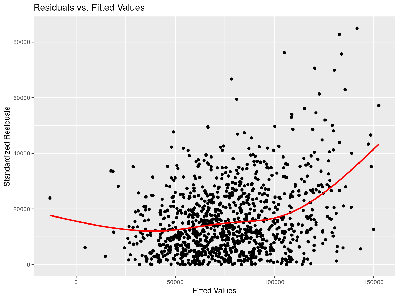
What is the biggest issue we haven’t tested for?
Spatial Autocorrelation!
Median Household Income clustering?
suppressPackageStartupMessages(require(spdep))
suppressPackageStartupMessages(require(spatialreg)) # This is new to me!
cbg_nb <- poly2nb(pl = cbg, queen = TRUE)
cbg_W <- nb2listw(cbg_nb,style="W")
cbg_moran_global <- moran.mc(x = cbg$mhi, listw = cbg_W, nsim=999,na.action = na.omit)
cbg_moran_global##
## Monte-Carlo simulation of Moran I
##
## data: cbg$mhi
## weights: cbg_W
## omitted: 230, 428, 432, 459, 471, 615, 640, 709, 782, 847, 942, 976
## number of simulations + 1: 1000
##
## statistic = 0.50705, observed rank = 1000, p-value = 0.001
## alternative hypothesis: greaterOur dependent variable (median household income) has positive spatial autocorrelation!
Looking at residuals
# Add in residuals
# We have to take into account lm() has dropped entries where any value is NA!
cbg$resid_lm[complete.cases(cbg %>% st_drop_geometry)] <- mod$residuals
tm_shape(cbg) +
tm_polygons(
col = 'resid_lm',
lwd = 0.2,
border.col = 'grey80',
title = "Error Quintiles (USD)",
palette = 'RdBu',
n=5,
midpoint = 0,
contrast =c(0,1),
style = 'quantile') +
tm_layout(main.title = 'Median Household Income - OLS Residuals')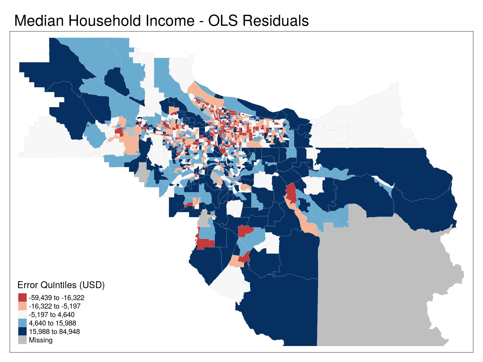
suppressMessages(tmap_mode('view'))
tmap_options(basemaps = c("Stamen.Toner",tmap_options()$basemaps))
tm_shape(cbg) +
tm_polygons(
col = 'resid_lm',
lwd = 0.2,
border.col = 'grey80',
title = "Error Quintiles (USD)",
palette = 'RdBu',
n=5,
alpha = 0.6,
midpoint = 0,
contrast =c(0,1),
style = 'quantile') +
tm_tiles("Stamen.TonerLabels") +
tm_layout(main.title = 'Median Household Income - OLS Residuals')Low values represent areas where our model overpredicted MHI, whereas high values are areas where our model underpredicted MHI
Clustering of residuals
##
## Monte-Carlo simulation of Moran I
##
## data: cbg$resid_lm
## weights: cbg_W
## omitted: 230, 428, 432, 459, 471, 530, 615, 640, 709, 782, 847, 942, 976
## number of simulations + 1: 1000
##
## statistic = 0.29454, observed rank = 1000, p-value = 0.001
## alternative hypothesis: greaterEven our residuals show significant clustering!
Wait, hold on!
What did we just do?
- Built a model for MHI
- Pulled the residuals (error) into our geographic data
- Mapped the geographic data, with colors representing error
We’re looking at a spatial representation of a statistical model’s accuracy!
If only we had a way to account for spatial autocorrelation in regression models…
Spatial Simultaneous Autoregressive Linear Models (Spatial Regression)
Standard Types
- Spatial Simultaneous Autoregressive Lag Model
- (Spatial Lag Model)
- Spatial Simultaneous Autoregressive Error Model
- (Spatial Error Model)
Ordinary Least Squares Regression
\[Y = \beta_0 + X_n\beta_n + \epsilon\]
where…
\(Y\) = Dependent Variable
\(\beta_0\) = Intercept
\(X_n\) = Independent Variable \(n\)
\(\beta_n\) = Coefficient \(n\)
\(\epsilon\) = Error term - assumed to be uncorrelated between two locations!
Spatial Lag Model
\[Y = \beta_0 + X\beta_n + \rho WY + \epsilon\]
where…
\(\rho WY\): autoregressive coefficient for the lag of the dependent variable
Spatial Error Model
\[Y = \beta_0 + X_n\beta_n + \lambda W\epsilon_A + \epsilon_R\]
where…
\(\lambda\) is a measure of the strength of autocorrelation in the error
\(W\) is the weight for two locations
\(\epsilon_A\) is the autoregressive portion of the error
\(\epsilon_R\) is the random portion of the error (there’s always error!)
General Process
General Process
- Identify your research question
- Look at your data
- Test for spatial autocorrelation
- Determine what type of model should be used (linear, spatial error/lag)
- Run model, assess results, make conclusions
Identify your research question
“Does educational attainment have an impact on median household income?”
Look at your data
Correlation - MHI and EDU
cbg %>% ggplot(aes(x=edu, y=mhi)) +
geom_point() +
geom_smooth(
method = 'lm',
formula = 'y ~ x') +
xlab("Educational Attainment") +
ylab("Median Household Income") +
ggtitle("Correlation of Variables")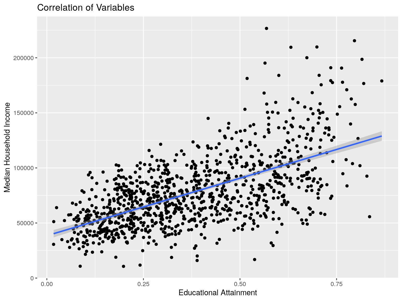
## [1] 0.6138181Correlation - MHI and HHS
cbg %>% ggplot(aes(x=hhs, y=mhi)) +
geom_point() +
geom_smooth(
method = 'lm',
formula = 'y ~ x') +
xlab("Household Size") +
ylab("Median Household Income") +
ggtitle("Correlation of Variables")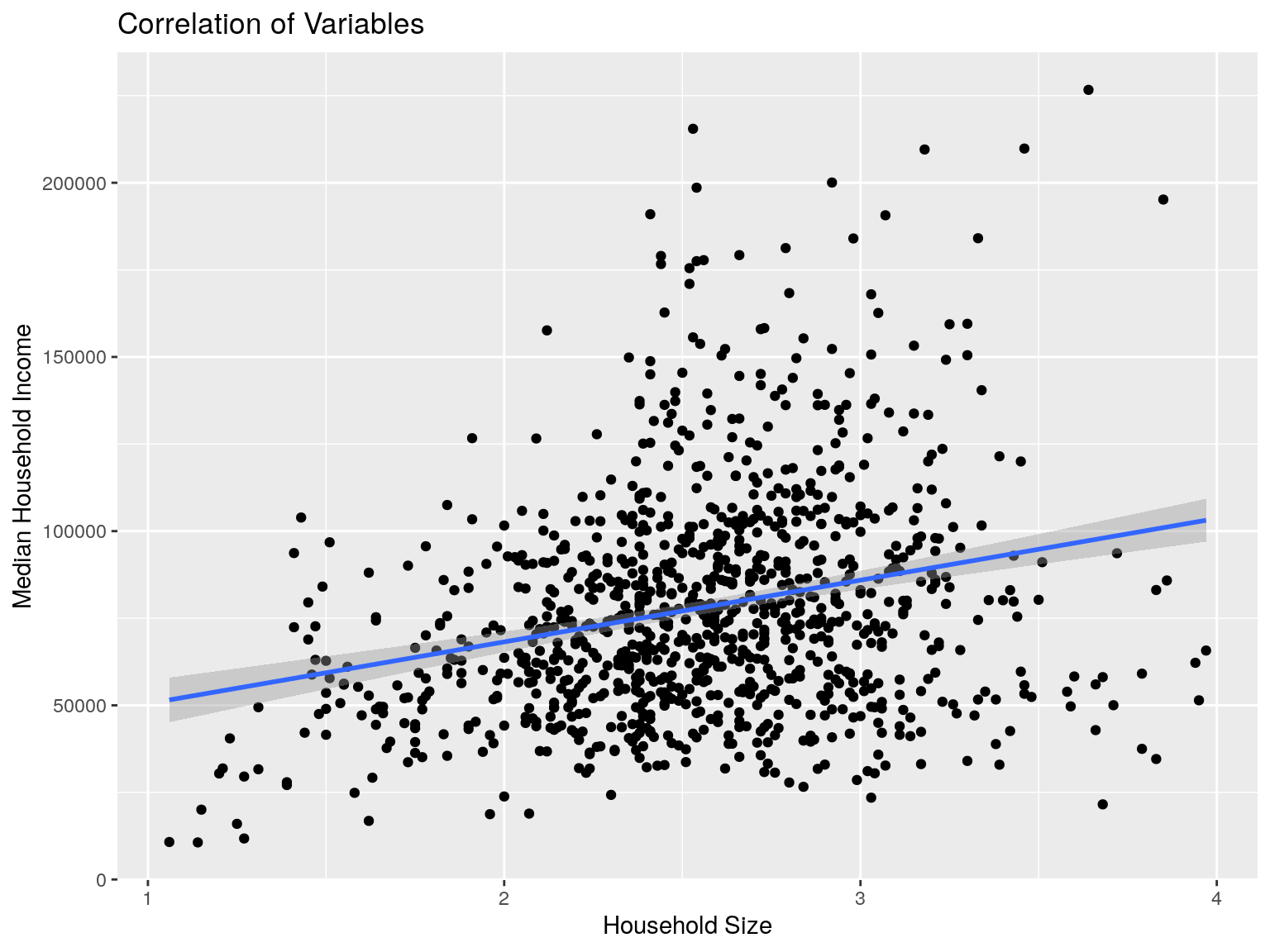
## [1] 0.2554926Correlation - EDU and HHS
cbg %>% ggplot(aes(x=hhs, y=edu)) +
geom_point() +
geom_smooth(
method = 'lm',
formula = 'y ~ x') +
xlab("Household Size") +
ylab("Educational Attainment") +
ggtitle("Correlation of Variables")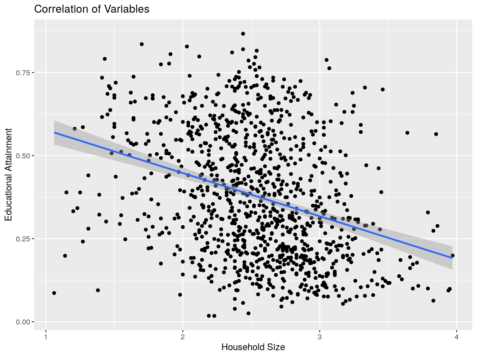
## [1] -0.3201357Distribution
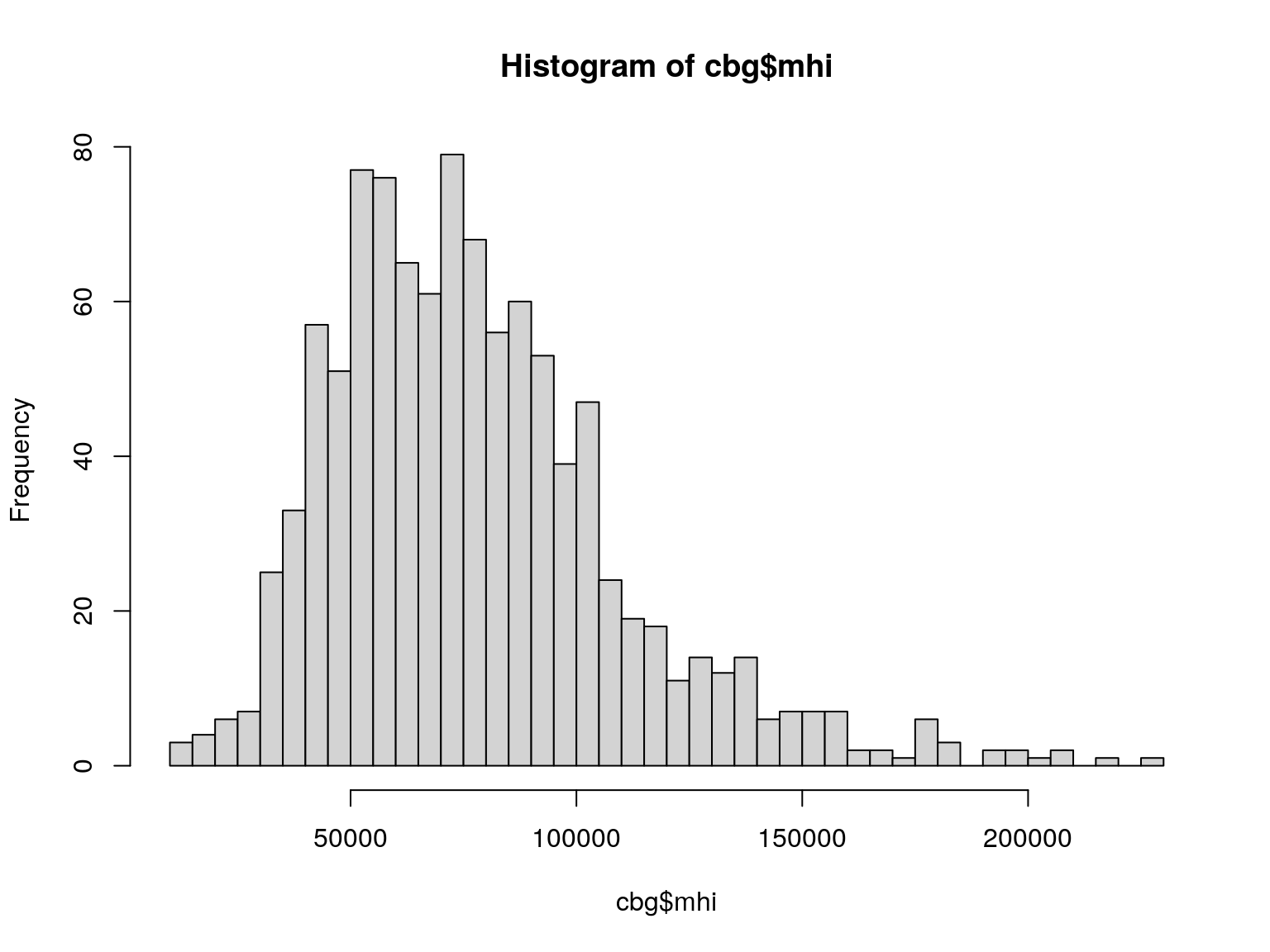
Log Distribution
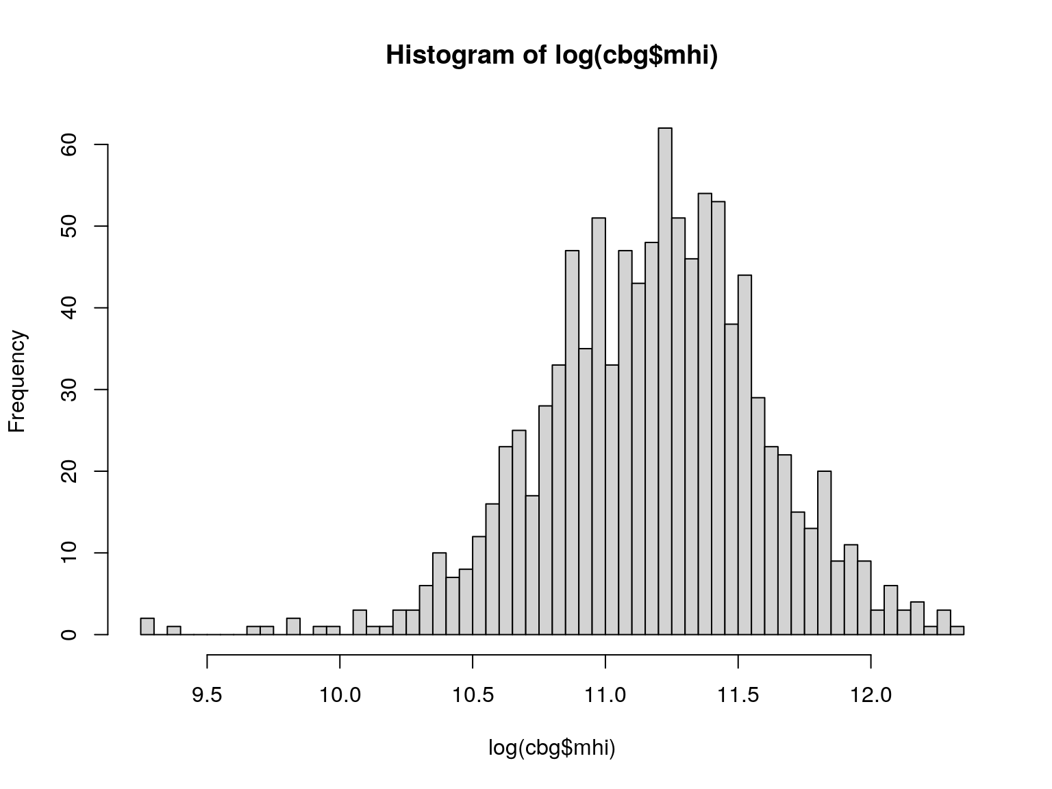
We can create a variable in our dataset for log(mhi)
Distribution
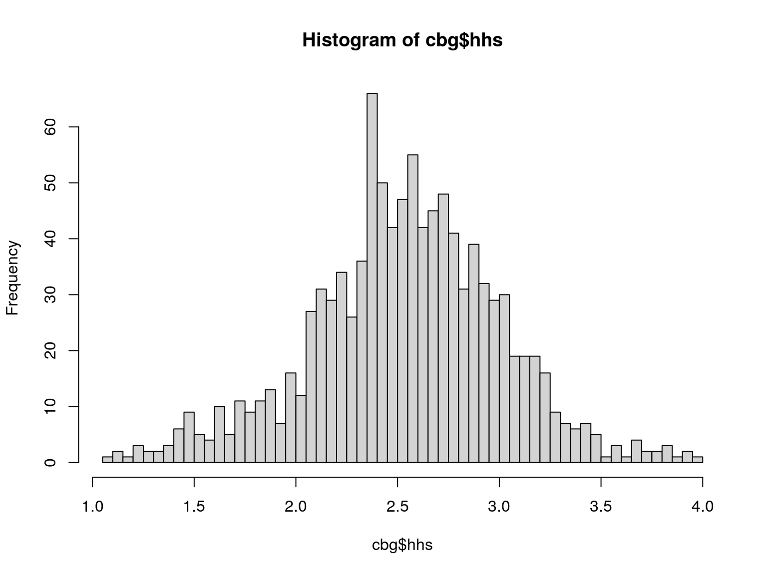
Distribution
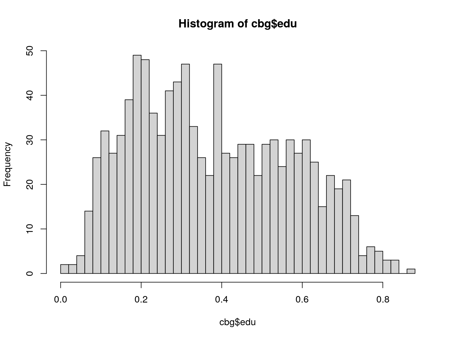
Test for Spatial Autocorrelation
We did this earlier
##
## Monte-Carlo simulation of Moran I
##
## data: cbg$mhi
## weights: cbg_W
## omitted: 230, 428, 432, 459, 471, 615, 640, 709, 782, 847, 942, 976
## number of simulations + 1: 1000
##
## statistic = 0.50705, observed rank = 1000, p-value = 0.001
## alternative hypothesis: greaterLet’s do it for log(mhi)
##
## Monte-Carlo simulation of Moran I
##
## data: cbg$log_mhi
## weights: cbg_W
## omitted: 230, 428, 432, 459, 471, 615, 640, 709, 782, 847, 942, 976
## number of simulations + 1: 1000
##
## statistic = 0.48017, observed rank = 1000, p-value = 0.001
## alternative hypothesis: greaterDetermine Model Type
Which to choose?
- Each model type is meant to be used on certain types of data
- Error: data with SA in error
- Lag: adjusting for spatial distribution of dependent variable
- We could calculate residual autocorrelation every time we alter a parameter, or…
Lagrange Multiplier
- Commonly used in non-spatial mathematics
- Used for optimization
- Function/parameter selection
- This can become complex.
- We’re geographers, we don’t want to be doing these calculations by hand
- Luckily, our friend Roger Bivand has made this simple for us in
spdep
Lagrange Multiplier
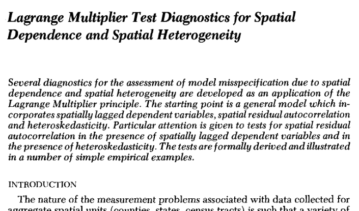
Lagrange Multiplier: spdep
First, we need to build a non-spatial OLS model!
##
## Call:
## lm(formula = log_mhi ~ edu + hhs, data = cbg)
##
## Residuals:
## Min 1Q Median 3Q Max
## -1.28276 -0.16608 0.02716 0.18399 0.70359
##
## Coefficients:
## Estimate Std. Error t value Pr(>|t|)
## (Intercept) 9.36067 0.05724 163.54 <2e-16 ***
## edu 1.66916 0.04659 35.83 <2e-16 ***
## hhs 0.46610 0.01900 24.53 <2e-16 ***
## ---
## Signif. codes: 0 '***' 0.001 '**' 0.01 '*' 0.05 '.' 0.1 ' ' 1
##
## Residual standard error: 0.2695 on 1025 degrees of freedom
## (13 observations deleted due to missingness)
## Multiple R-squared: 0.5891, Adjusted R-squared: 0.5883
## F-statistic: 734.9 on 2 and 1025 DF, p-value: < 2.2e-16Calculating VIF:
##      edu      hhs
## 1.117701 1.117701Looks good!
Now we run the test!
##
## Lagrange multiplier diagnostics for spatial dependence
##
## data:
## model: lm(formula = log_mhi ~ edu + hhs, data = cbg)
## weights: cbg_W
##
## LMerr = 243.66, df = 1, p-value < 2.2e-16
##
##
## Lagrange multiplier diagnostics for spatial dependence
##
## data:
## model: lm(formula = log_mhi ~ edu + hhs, data = cbg)
## weights: cbg_W
##
## LMlag = 199.98, df = 1, p-value < 2.2e-16
##
##
## Lagrange multiplier diagnostics for spatial dependence
##
## data:
## model: lm(formula = log_mhi ~ edu + hhs, data = cbg)
## weights: cbg_W
##
## RLMerr = 61.063, df = 1, p-value = 5.551e-15
##
##
## Lagrange multiplier diagnostics for spatial dependence
##
## data:
## model: lm(formula = log_mhi ~ edu + hhs, data = cbg)
## weights: cbg_W
##
## RLMlag = 17.385, df = 1, p-value = 3.052e-05
##
##
## Lagrange multiplier diagnostics for spatial dependence
##
## data:
## model: lm(formula = log_mhi ~ edu + hhs, data = cbg)
## weights: cbg_W
##
## SARMA = 261.04, df = 2, p-value < 2.2e-16Clean output with summary()
## Lagrange multiplier diagnostics for spatial dependence
## data:
## model: lm(formula = log_mhi ~ edu + hhs, data = cbg)
## weights: cbg_W
##
## statistic parameter p.value
## LMerr 243.659 1 < 2.2e-16 ***
## LMlag 199.981 1 < 2.2e-16 ***
## RLMerr 61.063 1 5.551e-15 ***
## RLMlag 17.385 1 3.052e-05 ***
## SARMA 261.044 2 < 2.2e-16 ***
## ---
## Signif. codes: 0 '***' 0.001 '**' 0.01 '*' 0.05 '.' 0.1 ' ' 1Which to select?
- Start with standard tests: which one has a significant p-value?
- If they’re both <= 0.05, look at the robust LM values.
- Choose the lowest robust
Both the Error and Lag LM values are significant.
statistic parameter p.value
LMerr 243.659 1 < 2.2e-16 ***
LMlag 199.981 1 < 2.2e-16 ***
RLMerr 61.063 1 5.551e-15 ***
RLMlag 17.385 1 3.052e-05 ***
SARMA 261.044 2 < 2.2e-16 ***
However, the robust Lagrange Multiplier value for the Error model is more significant!
statistic parameter p.value
LMerr 243.659 1 < 2.2e-16 ***
LMlag 199.981 1 < 2.2e-16 ***
RLMerr 61.063 1 5.551e-15 ***
RLMlag 17.385 1 3.052e-05 ***
SARMA 261.044 2 < 2.2e-16 ***
Model selection
We have concluded that a Spatial Error Model is the most appropriate for our data!
Run Model
Spatial Error Model
Almost as simple as a standard OLS model:
Error Model Results
##
## Call:spatialreg::errorsarlm(formula = formula, data = data, listw = listw,
## na.action = na.action, Durbin = Durbin, etype = etype, method = method,
## quiet = quiet, zero.policy = zero.policy, interval = interval,
## tol.solve = tol.solve, trs = trs, control = control)
##
## Residuals:
## Min 1Q Median 3Q Max
## -1.084497 -0.141398 0.015277 0.162513 0.722962
##
## Type: error
## Coefficients: (asymptotic standard errors)
## Estimate Std. Error z value Pr(>|z|)
## (Intercept) 9.652549 0.061550 156.826 < 2.2e-16
## edu 1.698418 0.062326 27.250 < 2.2e-16
## hhs 0.344817 0.019618 17.576 < 2.2e-16
##
## Lambda: 0.5942, LR test value: 202.14, p-value: < 2.22e-16
## Asymptotic standard error: 0.035131
## z-value: 16.914, p-value: < 2.22e-16
## Wald statistic: 286.08, p-value: < 2.22e-16
##
## Log likelihood: -8.23079 for error model
## ML residual variance (sigma squared): 0.055488, (sigma: 0.23556)
## Nagelkerke pseudo-R-squared: 0.66248
## Number of observations: 1028
## Number of parameters estimated: 5
## AIC: 26.462, (AIC for lm: 226.6)That’s a lot of information, let’s break it down…
Results: Coefficients
Estimate Std. Error z value Pr(>|z|) (Intercept) 9.652549 0.061550 156.826 < 2.2e-16 edu 1.698418 0.062326 27.250 < 2.2e-16 hhs 0.344817 0.019618 17.576 < 2.2e-16
- A 10% increase in adults 25+ with a college degree results in a 17% increase in Median Household Income
- A 1 person increase in household size results in a 34% increase in Median Household Income
Results: Error Parameter
Lambda: 0.5942, LR test value: 202.14, p-value: < 2.22e-16 Asymptotic standard error: 0.035131 z-value: 16.914, p-value: < 2.22e-16 Wald statistic: 286.08, p-value: < 2.22e-16
- Significant Lambda means that the introduction of Lambda is an improvement
- Wald statistic: similar to Lagrange Multiplier, a significant value states that the overall spatial model is likely an improvement over an OLS model
Results: Model Comparison
Log likelihood: -8.23079 for error model ML residual variance (sigma squared): 0.055488, (sigma: 0.23556) Nagelkerke pseudo-R-squared: 0.66248 Number of observations: 1028 Number of parameters estimated: 5 AIC: 26.462, (AIC for lm: 226.6)
- The log likelihood is valuable for comparing models
- The higher the value the better!
- Nagelkerke pseudo-R-squared is the best estimate for \(R^2\).
- Only useful when comparing other Nagelkerke \(R^2\)s!
- The Akaike information criterion accounts for model complexity.
- The lower the better!
What if we ran a Spatial Lag Model?
Lag: Summary
##
## Call:spatialreg::lagsarlm(formula = formula, data = data, listw = listw,
## na.action = na.action, Durbin = Durbin, type = type, method = method,
## quiet = quiet, zero.policy = zero.policy, interval = interval,
## tol.solve = tol.solve, trs = trs, control = control)
##
## Residuals:
## Min 1Q Median 3Q Max
## -1.214816 -0.147020 0.016532 0.167160 0.779488
##
## Type: lag
## Coefficients: (asymptotic standard errors)
## Estimate Std. Error z value Pr(>|z|)
## (Intercept) 5.055071 0.322998 15.650 < 2.2e-16
## edu 1.246928 0.056205 22.186 < 2.2e-16
## hhs 0.373731 0.018033 20.724 < 2.2e-16
##
## Rho: 0.42043, LR test value: 166.91, p-value: < 2.22e-16
## Asymptotic standard error: 0.03101
## z-value: 13.558, p-value: < 2.22e-16
## Wald statistic: 183.82, p-value: < 2.22e-16
##
## Log likelihood: -25.84458 for lag model
## ML residual variance (sigma squared): 0.059636, (sigma: 0.2442)
## Nagelkerke pseudo-R-squared: 0.65071
## Number of observations: 1028
## Number of parameters estimated: 5
## AIC: 61.689, (AIC for lm: 226.6)
## LM test for residual autocorrelation
## test value: 15.423, p-value: 8.5939e-05Lag: Impacts
- Lag coefficients are not directly interpretable
- We must consider the surrounding neighbors
- i has an impact on j… and j has an impact on i!
Lag: Impacts
spatialreg::impacts() can tell us a more complete story of spatial Lag coefficients. First we need to alter the weights matrix to remove zero-linked weights (lagsarlm did this for us):
Lag: Impacts
## Impact measures (lag, exact):
## Direct Indirect Total
## edu 1.2904099 0.8610496 2.1514595
## hhs 0.3867635 0.2580750 0.6448385Lag: Impacts
Direct Indirect Total
edu 1.2904099 0.8610496 2.1514595
hhs 0.3867635 0.2580750 0.6448385
- A 10% increase in adults 25+ with a college degree results in a 12.90% increase in Median Household Income in the observed polygon
- A 10% increase in adults 25+ with a college degree results in a 8.61% increase in Median Household Income in neighboring polygons
- A 10% increase in adults 25+ with a college degree results in a 21.51% total increase in Median Household Income
Lag: Impacts
Direct Indirect Total
edu 1.2904099 0.8610496 2.1514595
hhs 0.3867635 0.2580750 0.6448385
- A 1 person increase in household size results in a 3.87% increase in Median Household Income in the observed polygon
- A 1 person increase in household size results in a 2.58% increase in Median Household Income in neighboring polygons
- A 1 person increase in household size results in a 6.45% total increase in Median Household Income
Error vs. Lag
The previous lag exercise was just that: an exercise. We can compare it to the Error model to see which is best:
## df AIC
## mod_lag 5 61.68916
## mod_err 5 26.46158The Lagrange Multiplier test led us down the correct path! It told us before we began modeling that the Spatial Error Model would have better performance.
RMSE - a geography staple!
RMSE is the standard test statistic for geographic modeling:
## [1] 0.2355584This is like saying “Our model is accurate +/-0.24 log(MHI)”.
Additional analysis
Are the residuals still Spatially Autocorrelated?
Remember, we saw significant clustering of values in the OLS model residuals:
##
##  Monte-Carlo simulation of Moran I
##
## data:  cbg$resid_lm
## weights: cbg_W
## omitted: 230, 428, 432, 459, 471, 530, 615, 640, 709, 782, 847, 942, 976
## number of simulations + 1: 1000
##
## statistic = 0.29454, observed rank = 1000, p-value = 0.001
## alternative hypothesis: greaterWe can also test for this in the Error model:
##
## Monte-Carlo simulation of Moran I
##
## data: mod_err$residuals
## weights: cbg_W_sub
## number of simulations + 1: 1000
##
## statistic = -0.037667, observed rank = 21, p-value = 0.979
## alternative hypothesis: greaterWe fail to reject \(H_0\) - the spatial patterns in the error are gone!
Spatial Error Model Residuals
complete_records <- complete.cases(cbg %>% st_drop_geometry()) # define this first
# Place SEM residuals into the cbg object, where it is complete
cbg$resid_err <- ifelse(complete_records,mod_err$residuals,NA)
# build an OLS model to compare agains
mod_log <- lm(log(mhi) ~ edu + hhs, data =cbg)
# Place lm() residuals into the cbg object, where it is complete
cbg$lm_err <- ifelse(complete_records,mod_log$residuals,NA)tm_shape(cbg) +
tm_polygons(
col = c('resid_err','lm_err'),
lwd = 0.2,
border.col = 'grey80',
title = c("SEM Error Quintiles (USD)","OLS Error Quintiles (USD)"),
palette = 'RdBu',
n=5,
alpha = 0.6,
midpoint = 0,
contrast =c(0,1),
style = 'quantile') +
tm_tiles("Stamen.TonerLabels")Spatial Error Model Residuals
OLS Residuals
Heteroskedasticiy
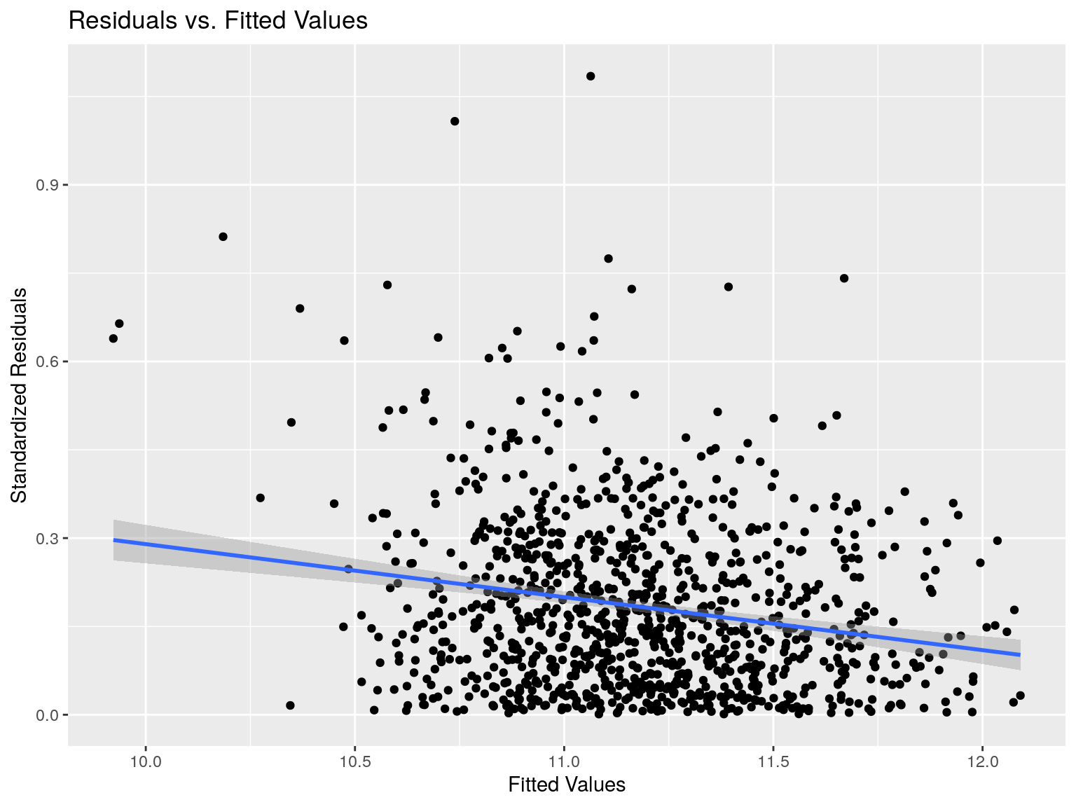
## [1] "R-squared: 0.0316"Looks random, which is a good sign!
Heteroskedasticiy
Alternatively, we have a more robust test for heteroskedasticity: The Breusch-Pagan test
##
## studentized Breusch-Pagan test
##
## data:
## BP = 25.334, df = 2, p-value = 3.153e-06We reject \(H_0\): heteroscedasticity is present! This is different than our ‘eyeballing’ last slide.
What do we do when there is heteroscedasticity?
- We can adjust for that
- Beyond scope of this class, though you may check out
?bptest.sarlm()for more info
- Beyond scope of this class, though you may check out
- We can introduce new variables to help
- a map help us think of new variables!
- We can acknowledge and accept that there are likely additional variables we are not accounting for
Interpretation
There is still potential local clustering, but we have resolved enough to account for spatial autocorrelation in our regression model!
Another Method
Error Recap
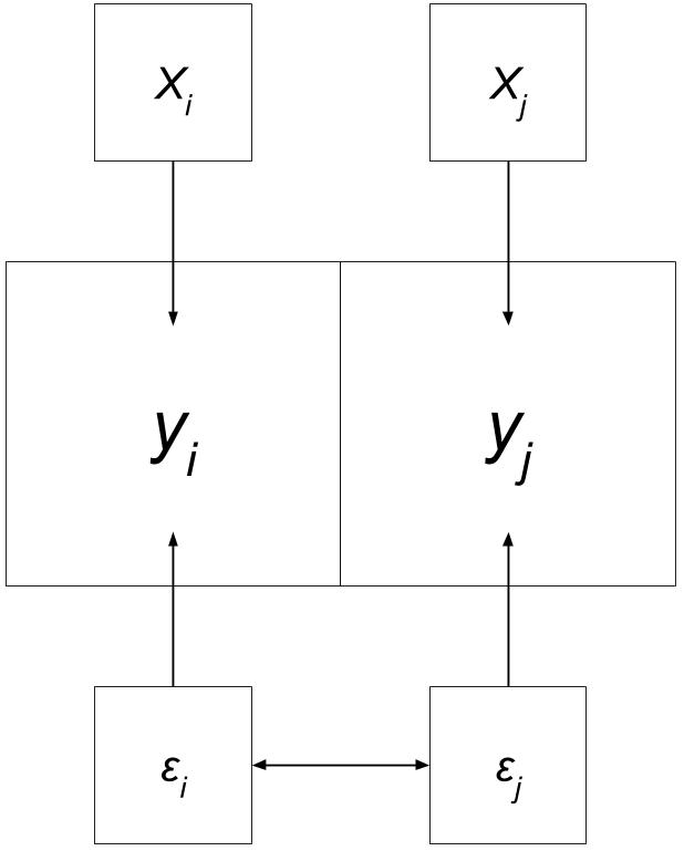
“Error terms across different spatial units are correlated.”
Adapted from “Spatial Regression with GeoDa”
Lag Recap
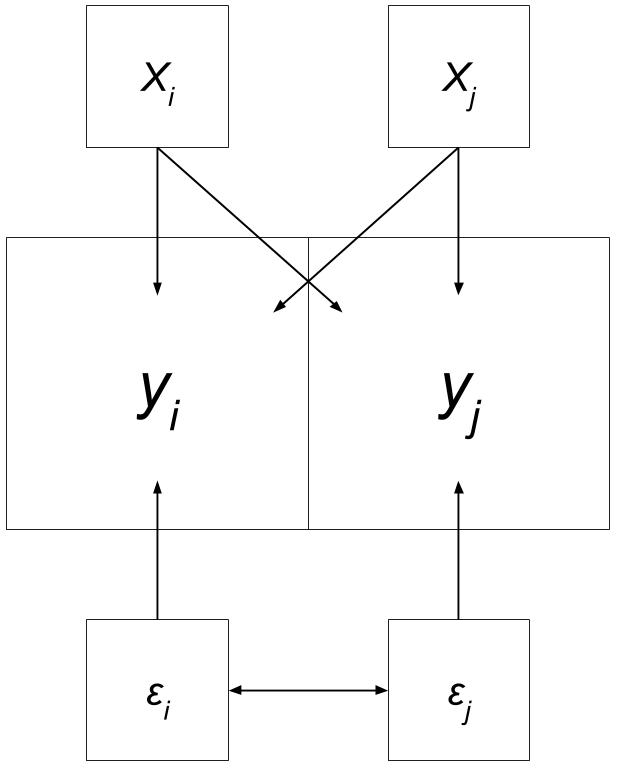
“Variable y in place i is affected by the independent variables in both place i and j.”
Adapted from “Spatial Regression with GeoDa”
But what if…
… we looked at everything in relation to everything else?
Spatial Durbin Model
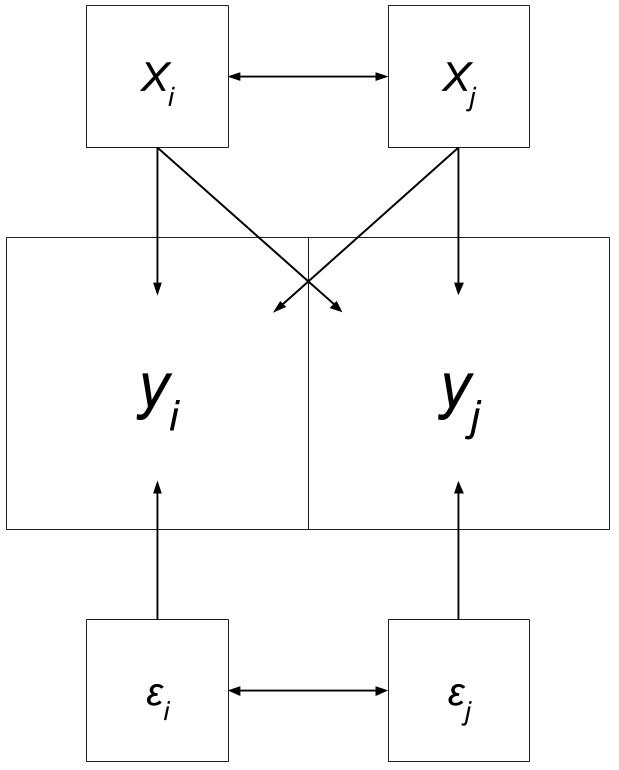
“Variable y in place i is affected by the independent variables in both place i and j, as well as the lag for the independent variables in both place i and j.”

Spatial Durbin Model
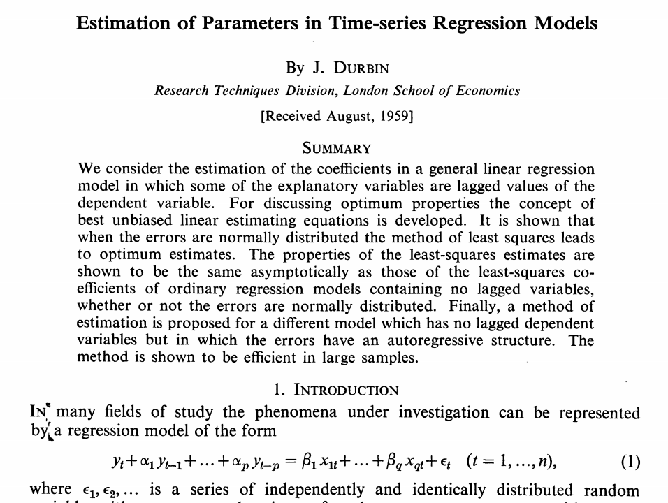
https://www.jstor.org/stable/2983884?seq=1#metadata_info_tab_contents
When do we use Durbin?
When we know there are:
- missing variables
- significant inter-neighborhood patterns
- significant clustering through a large amount of our independent variables
- when our research question depends on it
When do we use Durbin?
Basically…
IT DEPENDS
Running the Model
mod_durbin <- spatialreg::lagsarlm(
formula = log_mhi ~ edu + hhs,
data = cbg, # the entire object
listw = cbg_W,
na.action = na.omit,
type = "Durbin"
)All we have to do is add type = "Durbin" to lagsarlm()!
##
## Call:spatialreg::lagsarlm(formula = formula, data = data, listw = listw,
## na.action = na.action, Durbin = Durbin, type = type, method = method,
## quiet = quiet, zero.policy = zero.policy, interval = interval,
## tol.solve = tol.solve, trs = trs, control = control)
##
## Residuals:
## Min 1Q Median 3Q Max
## -1.0791339 -0.1341632 0.0081202 0.1595892 0.8007955
##
## Type: mixed
## Coefficients: (asymptotic standard errors)
## Estimate Std. Error z value Pr(>|z|)
## (Intercept) 4.227153 0.353636 11.9534 < 2.2e-16
## edu 1.759111 0.073700 23.8686 < 2.2e-16
## hhs 0.318782 0.019940 15.9868 < 2.2e-16
## lag.edu -0.839124 0.114354 -7.3379 2.169e-13
## lag.hhs 0.032655 0.038075 0.8576 0.3911
##
## Rho: 0.51058, LR test value: 159.94, p-value: < 2.22e-16
## Asymptotic standard error: 0.03848
## z-value: 13.269, p-value: < 2.22e-16
## Wald statistic: 176.06, p-value: < 2.22e-16
##
## Log likelihood: 17.32267 for mixed model
## ML residual variance (sigma squared): 0.053896, (sigma: 0.23215)
## Nagelkerke pseudo-R-squared: 0.67885
## Number of observations: 1028
## Number of parameters estimated: 7
## AIC: -20.645, (AIC for lm: 137.29)
## LM test for residual autocorrelation
## test value: 39.571, p-value: 3.1631e-10Comparison: AIC
##         df      AIC
## mod_lag  5 61.68916
## mod_err  5 26.46158
## mod_durbin 7 -20.64534The Spatial Durbin Model may be our best bet, even when accounting for the added complexity!
Comparison: Nagelkerke R-squared
lapply(
  X = list(mod_err,mod_lag,mod_durbin),
  function(i) data.frame(model = i$type, `NK R2` = summary(i,Nagelkerke=T)$NK)
  ) %>% invisible() %>%
  bind_rows()
## model NK.R2
## 1 error 0.6624771
## 2 lag 0.6507103
## 3 mixed 0.6788467Again, our Nagelkerke R-squared shows that the Durbin model is likely explaining the most variance in Median Household Income.
Durbin: Impacts
## Impact measures (mixed, exact):
##        Direct  Indirect     Total
## edu 1.7655436 0.1142066 1.8797502
## hhs 0.3400725 0.3779974 0.7180699
Spatial Durbin Model Residuals
cbg$resid_dur <- ifelse(!is.na(cbg$resid_err), mod_durbin$residuals,NA)

tm_shape(cbg) +
  tm_polygons(
    col = 'resid_dur',
    lwd = 0.2,
    border.col = 'grey80',
    title = "Durbin Error Quintiles (USD)",
    palette = 'RdBu',
    n=5,
    alpha = 0.6,
    midpoint = 0,
    contrast =c(0,1),
    style = 'quantile') +
  tm_tiles("Stamen.TonerLabels")
Spatial Durbin Model Residuals
Spatial Error Model Residuals
Next Class
Final Project Discussion
Send me a DM on Slack telling me what you’d like to present on! Include the following, as best you can:
- Hypothesis
- Data sources
- Planned analysis
Lab
- Spatial Regression
- This will take a fair amount of time… but will likely overlap with your final!