Spatial Analysis and Spatial Data
GEOG 4/597: Advanced Spatial Quantitative
Analysis, Winter 2023
Jackson Voelkel | Portland State
University
Overview
- Define Spatial Analysis
- Review the entity-attribute model
- Distinguish spatial analysis from GIS-based analysis
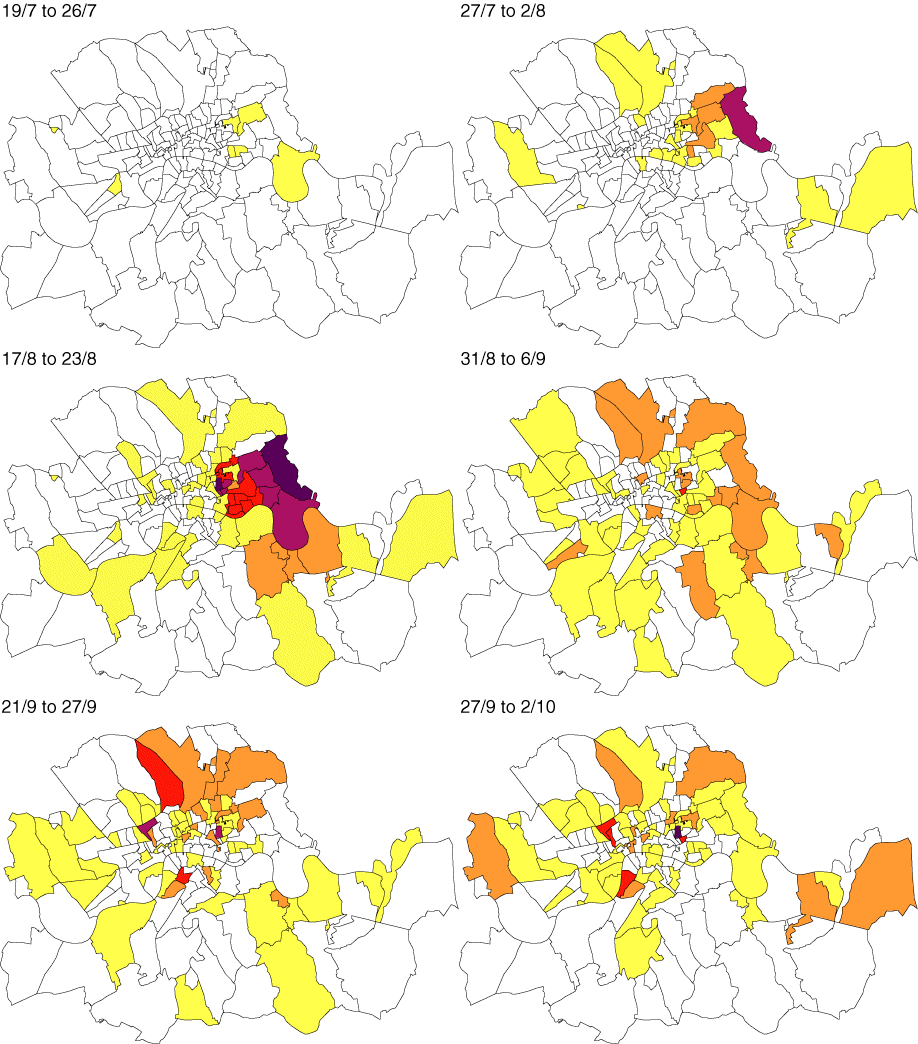
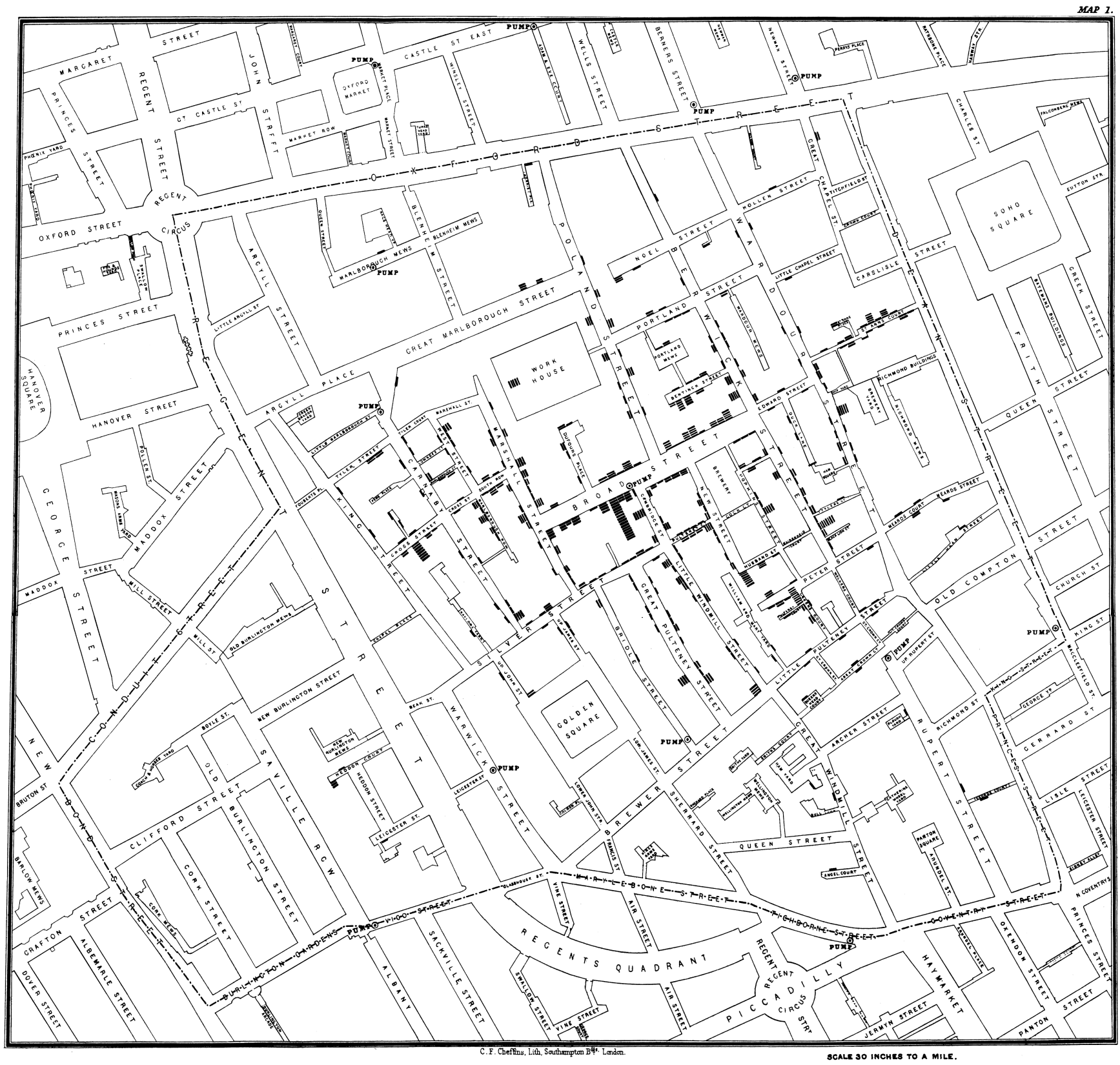
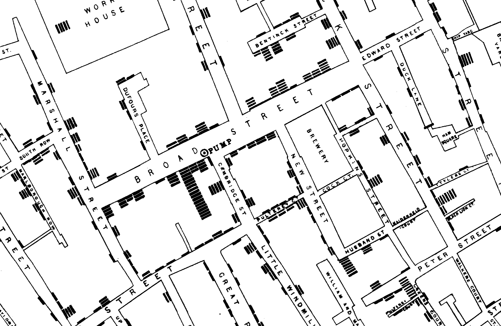
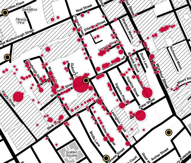
When a Map Changed the World: John Snow’s Cholera Study
NO
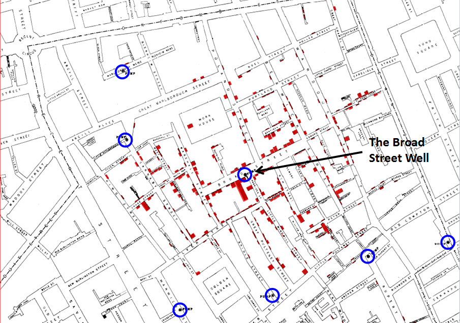
- Cholera outbreak on Broad Street in Soho London in 1854
- On the Mode of Communication of Cholera in 1849 and 1855
- Predates understanding and acceptance of bacteriology and germ theory

http://ecodevoevo.blogspot.com/2014/10/was-john-snow-more-of-empiricist-than.html

Voronoi Diagrams
AKA Thiessen Polygons
Numerous polygons are created:
- Each polygon contains a point, \(p_K\)
- Its corresponding polygon consists of every point whose distance to \(p_K\) is less than or equal to the distance to any other \(p_K\)
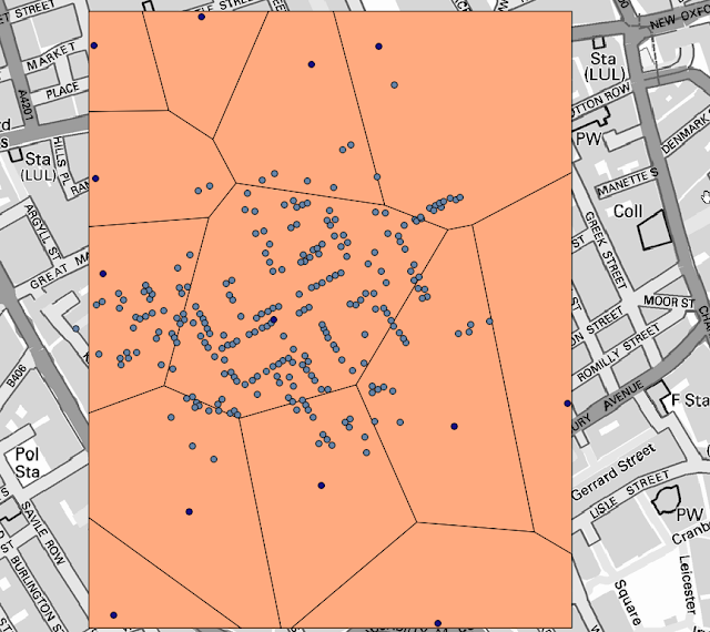
http://qgissextante.blogspot.com/2012/10/analyzing-john-snows-cholera-dataset.html
Spatial Allocation: walking distance
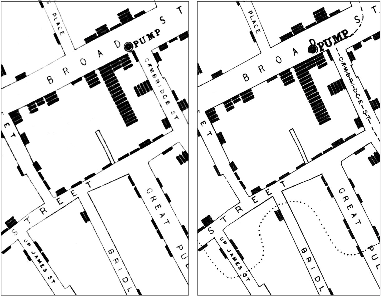
Dotted line: the map on the right is a later version.
https://johnsnow.matrix.msu.edu/images/online_companion/chapter_images/fig12-7.jpg
John Snow’s Cholera Study
- Snow had a hypothesis that cholera was a waterborne disease before he even drew his maps
- Spatial analysis did not prove his theory. That required microbiology and pathology (in 1883, Rober Kock isolated Vibrio cholerae).
- But … spatial analysis did provide supporting evidence that had an important impact on policy.
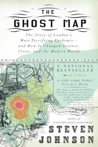
Steven Johnson
The Ghost Map: Story of London’s Most Terrifying Epidemic - and How It Changed Science, Cities, and the Modern World
Spatial Analysis
Spatial Analysis is concerned with investigating the patterns that arise as a result of processes that may be operating in space. Techniques and methods to enable the representation, description, measurement, comparison and generation of spatial patterns are central to the study of geographic information analysis.
O’Sullivan and Unwin, page 4
Four Types of Spatial Analysis
- Spatial data manipulation
- Spatial data analysis
- Spatial statistical analysis
- Spatial Modeling
1: Spatial data manipulation
- Typically done via GIS
- E.g., merging, overlay, dissolve.
2: Spatial data analysis
- First steps in analysis: exploratory and descriptive
3: Spatial statistical analysis
- Hypothesis testing
4: Spatial Modeling
- Forecasts and predictions
- E.g., climate change modeling
What will we do?
2 Spatial data analysis
3 Spatial statistical analysis
4
Spatial Modeling
That is a lot, considering how long you’ve studied just #1 (and maybe a bit of #2)
Spatial Data Analysis
Spatial data analysis is concerned with that branch of data analysis where the geographical referencing of objects contains important information. In many areas of data collection, especially in some areas of experimental science, the indexes that distinguish different cases can be exchanged without any loss of information. All the information relevant to understanding the variation in the data set is contained in the observations and no relevant information is contained in the indexing. In the case of spatial data the indexing (by location and time) may contain crucial information. A definition of spatial analysis (of which spatial data analysis is one element) is that it represents a collection of techniques and models that explicitly use the spatial referencing of each data case.
Goodchild, Michael, and Haining. 2004. “GIS and spatial data analysis: converging perspectives”. Papers in Regional Science 83:363-385
Spatial Data - A refresher
- What are spatial data?
- How do we represent the world in GIS?
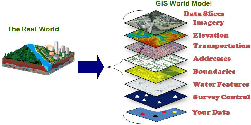
www.in.gov/gis/gis101.htm
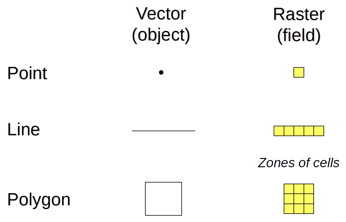
Vector (object) vs. Raster (field)
- Vector (object): Describes the world as a space filled with discrete, identifiable units that have some type of spatial reference
- Raster (field): Describes the world as a collection of continuous spatial distributions of different phenomena
Vector (object) vs. Raster (field)
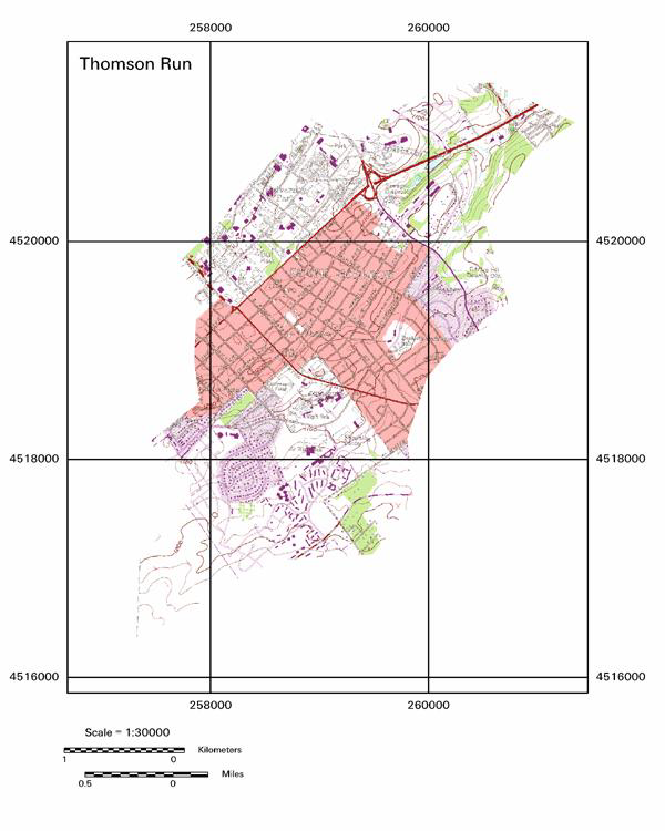
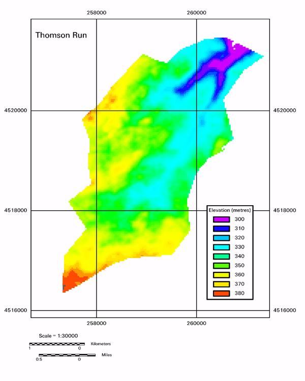
Raster and Vector Data
Fields
- Useful when the phenomenon is measured at all locations … such as?
- Common in physical geography
- Often used to visualize patterns
- Usually represented on a grid

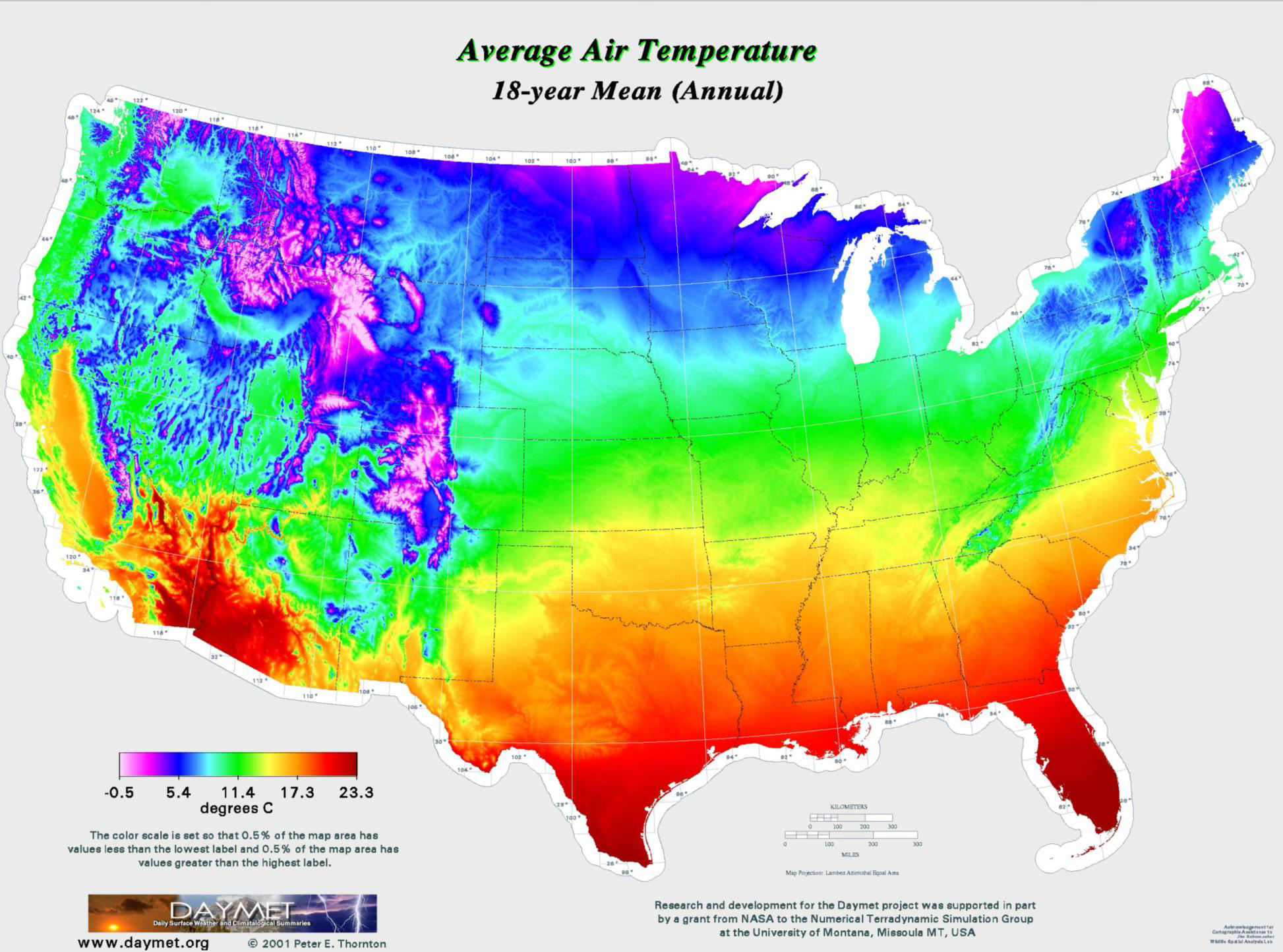
Can you name this location? Hint: it is very close to downtown Portland!
An example in R
require(raster)
require(tmap)
rgbi <- stack('C:/data/rgbi.tif') %>%
  `names()<-`(c("R","G","B","I"))

dhm <- raster('C:/data/dhm.tif')

dhm
rgbi
## class : RasterLayer
## dimensions : 948, 1005, 952740 (nrow, ncol, ncell)
## resolution : 3, 3 (x, y)
## extent : 744597.5, 747612.5, 1379506, 1382350 (xmin, xmax, ymin, ymax)
## crs : +proj=lcc +lat_0=41.75 +lon_0=-120.5 +lat_1=43 +lat_2=45.5 +x_0=400000 +y_0=0 +ellps=GRS80 +units=ft +no_defs
## source : dhm.tif
## names : dhm
## values : 0, 203.74 (min, max)## class : RasterStack
## dimensions : 948, 1005, 952740, 4 (nrow, ncol, ncell, nlayers)
## resolution : 3, 3 (x, y)
## extent : 744597.5, 747612.5, 1379506, 1382350 (xmin, xmax, ymin, ymax)
## crs : +proj=lcc +lat_0=41.75 +lon_0=-120.5 +lat_1=43 +lat_2=45.5 +x_0=400000 +y_0=0 +ellps=GRS80 +units=ft +no_defs
## names : R, G, B, IRGBI
tmap_options(legend.outside=T,legend.outside.size = 0.2)
tm_shape(rgbi) +
  tm_rgb(r = 4,g = 2,b = 3) +
  tm_layout(main.title = "False Color Infrared")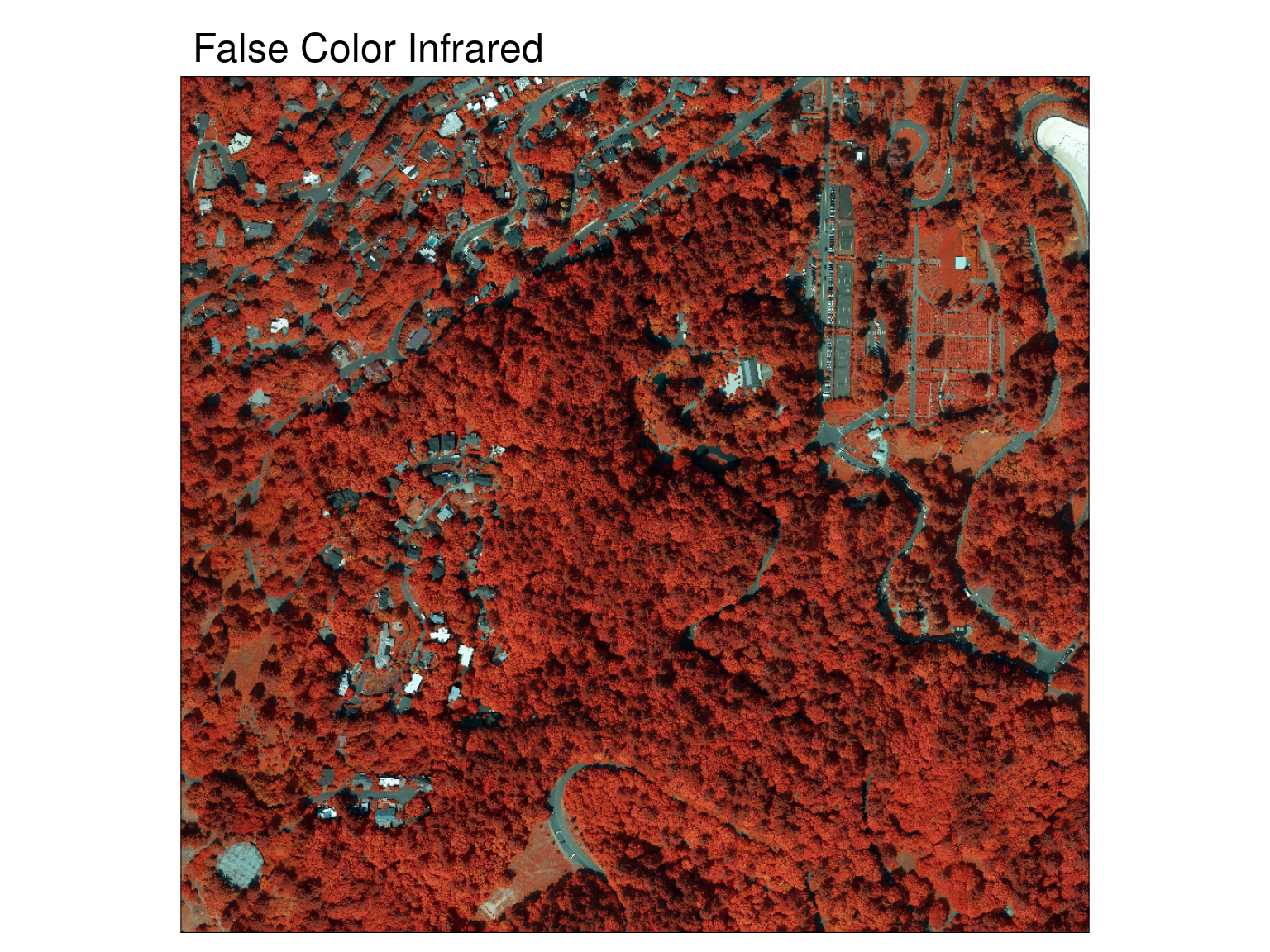
DHM
tm_shape(dhm) +
  tm_raster(style = 'cont',title="Height",palette = "-Greys") +
  tm_layout(main.title = "Digital Height Model",outer.margins = c(0.01,0.03,0.03,-0.1))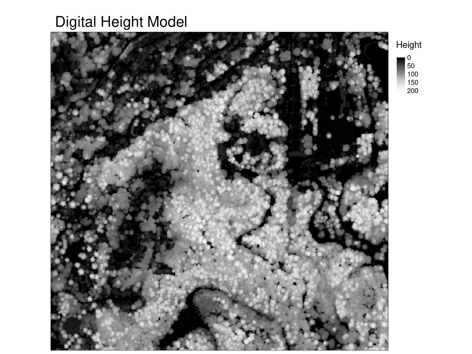
Convert to a dataframe
##      R  G  B   I
## 1   56 65 51 140
## 2   34 42 31 113
## 3   36 44 34 127
## 4   15 19 15  79
## 5    3  6  9  41
## 6    3  5  9  33
## 7    3  5  7  31
## 8    8 14 16  56
## 9   22 32 31 100
## 10   6 11 11  52
## 11   3  6  9  36
## 12   3  7  9  44
## 13   3  6 10  44
## 14   4  9 12  46
## 15   3  5 10  43
## 16  34 45 36 143
## 17  34 44 29 138
## 18  50 65 45 177
## 19  41 53 38 166
## 20  12 15 10  94
## 21  59 75 52 191
## 22  38 49 32 162
## 23  50 64 45 177
## 24  36 48 32 146
## 25  26 36 26 120
## 26  46 62 51 170
## 27  26 35 25 120
## 28  20 27 18  94
## 29  65 78 60 162
## 30  53 62 48 139
## 31  38 46 33 119
## 32  56 65 48 135
## 33  66 79 62 148
## 34  70 77 59 138
## 35  20 25 17  68
## 36  10 15 11  52
## 37   8 13 11  46
## 38   6 10 11  39
## 39  13 18 15  61
## 40  29 36 26 103
## 41  29 37 24 113
## 42  14 22 16  90
## 43  12 19 17  77
## 44  11 18 17  79
## 45  36 47 36 139
## 46   7 11  9  61
## 47  40 53 38 133
## 48   6 10 13  13
## 49   5  9 14   7
## 50   5 10 15   5
## 51   7 12 18   8
## 52   6 12 16   6
## 53   7 10 17   7
## 54  11 16 22  10
## 55  25 27 32  19
## 56  50 48 48  39
## 57  15 16 14  13
## 58  83 79 77  66
## 59  84 80 77  60
## 60  81 78 76  59
## 61  75 71 71  52
## 62  70 67 67  55
## 63  65 57 52  65
## 64  60 51 48  58
## 65  64 52 48  66
## 66  63 54 50  64
## 67  60 53 51  59
## 68  38 35 38  37
## 69  15 16 21  24
## 70   8 12 14  31
## 71  43 54 32 135
## 72  70 82 50 185
## 73  64 72 45 175
## 74  39 53 34 171
## 75  44 60 39 169
## 76  42 55 40 174
## 77  32 46 28 159
## 78  46 65 35 173
## 79  24 36 18 116
## 80  33 44 26 115
## 81  30 40 29 109
## 82  61 73 57 149
## 83  56 68 53 145
## 84  46 57 44 128
## 85  37 47 38 113
## 86  61 74 61 149
## 87  57 72 56 143
## 88  64 77 61 153
## 89  55 68 51 147
## 90  56 67 55 135
## 91  50 62 51 138
## 92  44 56 47 128
## 93  45 55 44 120
## 94  37 48 38 118
## 95  48 60 48 132
## 96  62 75 59 149
## 97  52 64 50 133
## 98  64 79 65 154
## 99  63 79 65 153
## 100 59 75 61 151
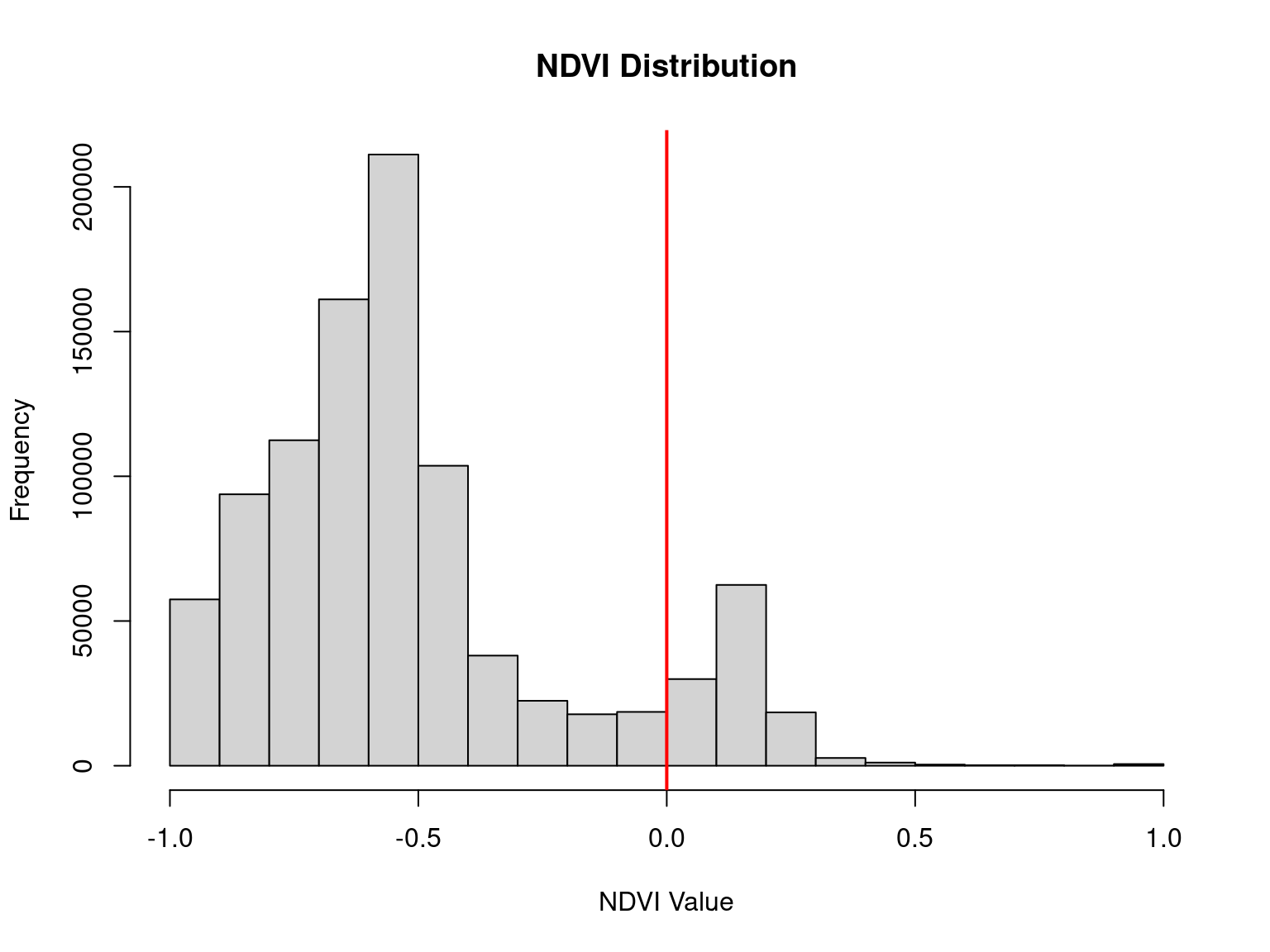
Create NDVI in the dataframe
\(NDVI = \frac{Red - NIR}{Red + NIR}\)
##      R  G  B   I         NDVI
## 1   56 65 51 140 -0.428571429
## 2   34 42 31 113 -0.537414966
## 3   36 44 34 127 -0.558282209
## 4   15 19 15  79 -0.680851064
## 5    3  6  9  41 -0.863636364
## 6    3  5  9  33 -0.833333333
## 7    3  5  7  31 -0.823529412
## 8    8 14 16  56 -0.750000000
## 9   22 32 31 100 -0.639344262
## 10   6 11 11  52 -0.793103448
## 11   3  6  9  36 -0.846153846
## 12   3  7  9  44 -0.872340426
## 13   3  6 10  44 -0.872340426
## 14   4  9 12  46 -0.840000000
## 15   3  5 10  43 -0.869565217
## 16  34 45 36 143 -0.615819209
## 17  34 44 29 138 -0.604651163
## 18  50 65 45 177 -0.559471366
## 19  41 53 38 166 -0.603864734
## 20  12 15 10  94 -0.773584906
## 21  59 75 52 191 -0.528000000
## 22  38 49 32 162 -0.620000000
## 23  50 64 45 177 -0.559471366
## 24  36 48 32 146 -0.604395604
## 25  26 36 26 120 -0.643835616
## 26  46 62 51 170 -0.574074074
## 27  26 35 25 120 -0.643835616
## 28  20 27 18  94 -0.649122807
## 29  65 78 60 162 -0.427312775
## 30  53 62 48 139 -0.447916667
## 31  38 46 33 119 -0.515923567
## 32  56 65 48 135 -0.413612565
## 33  66 79 62 148 -0.383177570
## 34  70 77 59 138 -0.326923077
## 35  20 25 17  68 -0.545454545
## 36  10 15 11  52 -0.677419355
## 37   8 13 11  46 -0.703703704
## 38   6 10 11  39 -0.733333333
## 39  13 18 15  61 -0.648648649
## 40  29 36 26 103 -0.560606061
## 41  29 37 24 113 -0.591549296
## 42  14 22 16  90 -0.730769231
## 43  12 19 17  77 -0.730337079
## 44  11 18 17  79 -0.755555556
## 45  36 47 36 139 -0.588571429
## 46   7 11  9  61 -0.794117647
## 47  40 53 38 133 -0.537572254
## 48   6 10 13  13 -0.368421053
## 49   5  9 14   7 -0.166666667
## 50   5 10 15   5  0.000000000
## 51   7 12 18   8 -0.066666667
## 52   6 12 16   6  0.000000000
## 53   7 10 17   7  0.000000000
## 54  11 16 22  10  0.047619048
## 55  25 27 32  19  0.136363636
## 56  50 48 48  39  0.123595506
## 57  15 16 14  13  0.071428571
## 58  83 79 77  66  0.114093960
## 59  84 80 77  60  0.166666667
## 60  81 78 76  59  0.157142857
## 61  75 71 71  52  0.181102362
## 62  70 67 67  55  0.120000000
## 63  65 57 52  65  0.000000000
## 64  60 51 48  58  0.016949153
## 65  64 52 48  66 -0.015384615
## 66  63 54 50  64 -0.007874016
## 67  60 53 51  59  0.008403361
## 68  38 35 38  37  0.013333333
## 69  15 16 21  24 -0.230769231
## 70   8 12 14  31 -0.589743590
## 71  43 54 32 135 -0.516853933
## 72  70 82 50 185 -0.450980392
## 73  64 72 45 175 -0.464435146
## 74  39 53 34 171 -0.628571429
## 75  44 60 39 169 -0.586854460
## 76  42 55 40 174 -0.611111111
## 77  32 46 28 159 -0.664921466
## 78  46 65 35 173 -0.579908676
## 79  24 36 18 116 -0.657142857
## 80  33 44 26 115 -0.554054054
## 81  30 40 29 109 -0.568345324
## 82  61 73 57 149 -0.419047619
## 83  56 68 53 145 -0.442786070
## 84  46 57 44 128 -0.471264368
## 85  37 47 38 113 -0.506666667
## 86  61 74 61 149 -0.419047619
## 87  57 72 56 143 -0.430000000
## 88  64 77 61 153 -0.410138249
## 89  55 68 51 147 -0.455445545
## 90  56 67 55 135 -0.413612565
## 91  50 62 51 138 -0.468085106
## 92  44 56 47 128 -0.488372093
## 93  45 55 44 120 -0.454545455
## 94  37 48 38 118 -0.522580645
## 95  48 60 48 132 -0.466666667
## 96  62 75 59 149 -0.412322275
## 97  52 64 50 133 -0.437837838
## 98  64 79 65 154 -0.412844037
## 99  63 79 65 153 -0.416666667
## 100 59 75 61 151 -0.438095238
Looks like we created NDVI correctly
Let’s make a model!
Linear/OLS models are very easy in R:
##
## Call:
## lm(formula = mpg ~ hp + wt, data = mtcars)
##
## Residuals:
##    Min     1Q Median     3Q    Max
## -3.941 -1.600 -0.182  1.050  5.854
##
## Coefficients:
##             Estimate Std. Error t value Pr(>|t|)
## (Intercept) 37.22727    1.59879  23.285  < 2e-16 ***
## hp          -0.03177    0.00903  -3.519  0.00145 **
## wt          -3.87783    0.63273  -6.129 1.12e-06 ***
## ---
## Signif. codes:  0 '***' 0.001 '**' 0.01 '*' 0.05 '.' 0.1 ' ' 1
##
## Residual standard error: 2.593 on 29 degrees of freedom
## Multiple R-squared:  0.8268, Adjusted R-squared:  0.8148
## F-statistic: 69.21 on 2 and 29 DF,  p-value: 9.109e-12
“MPG as a function of Horsepower and Weight”
Let’s make a model!
Our raster data is also now a data.frame!
##
## Call:
## lm(formula = dhm_df$dhm ~ rgbi_df$NDVI)
##
## Residuals:
##      Min       1Q   Median       3Q      Max
## -108.801  -27.089    0.794   27.809  158.684
##
## Coefficients:
##               Estimate Std. Error t value Pr(>|t|)
## (Intercept)   23.24802    0.07695   302.1   <2e-16 ***
## rgbi_df$NDVI -85.55340    0.12767  -670.1   <2e-16 ***
## ---
## Signif. codes:  0 '***' 0.001 '**' 0.01 '*' 0.05 '.' 0.1 ' ' 1
##
## Residual standard error: 39.03 on 952386 degrees of freedom
##   (352 observations deleted due to missingness)
## Multiple R-squared:  0.3204, Adjusted R-squared:  0.3204
## F-statistic: 4.49e+05 on 1 and 952386 DF,  p-value: < 2.2e-16
Wouldn’t it be great if we could see where our model error is?
Plotting Residuals
tm_shape(resid) +
  tm_raster(style = "cont", palette = "RdBu",title = "Residuals") +
  tm_layout(main.title = "Residual Map",outer.margins = c(0.01,0.03,0.03,-0.03))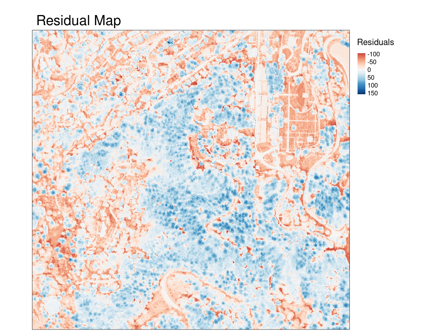
So… what are we looking at?
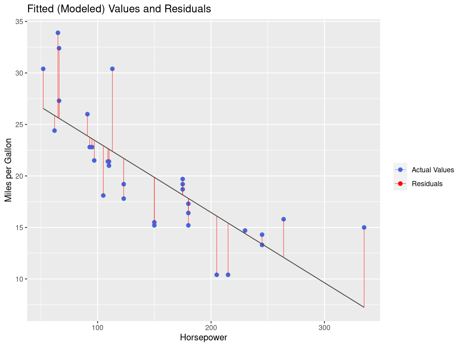
Residuals Refresher
Predicting With a Model
tm_shape(dhm_model) +
  tm_raster(style = "cont", palette = "-Greys",title = "Height") +
  tm_layout(main.title = "Predicted Heights",outer.margins = c(0.01,0.03,0.03,-0.03))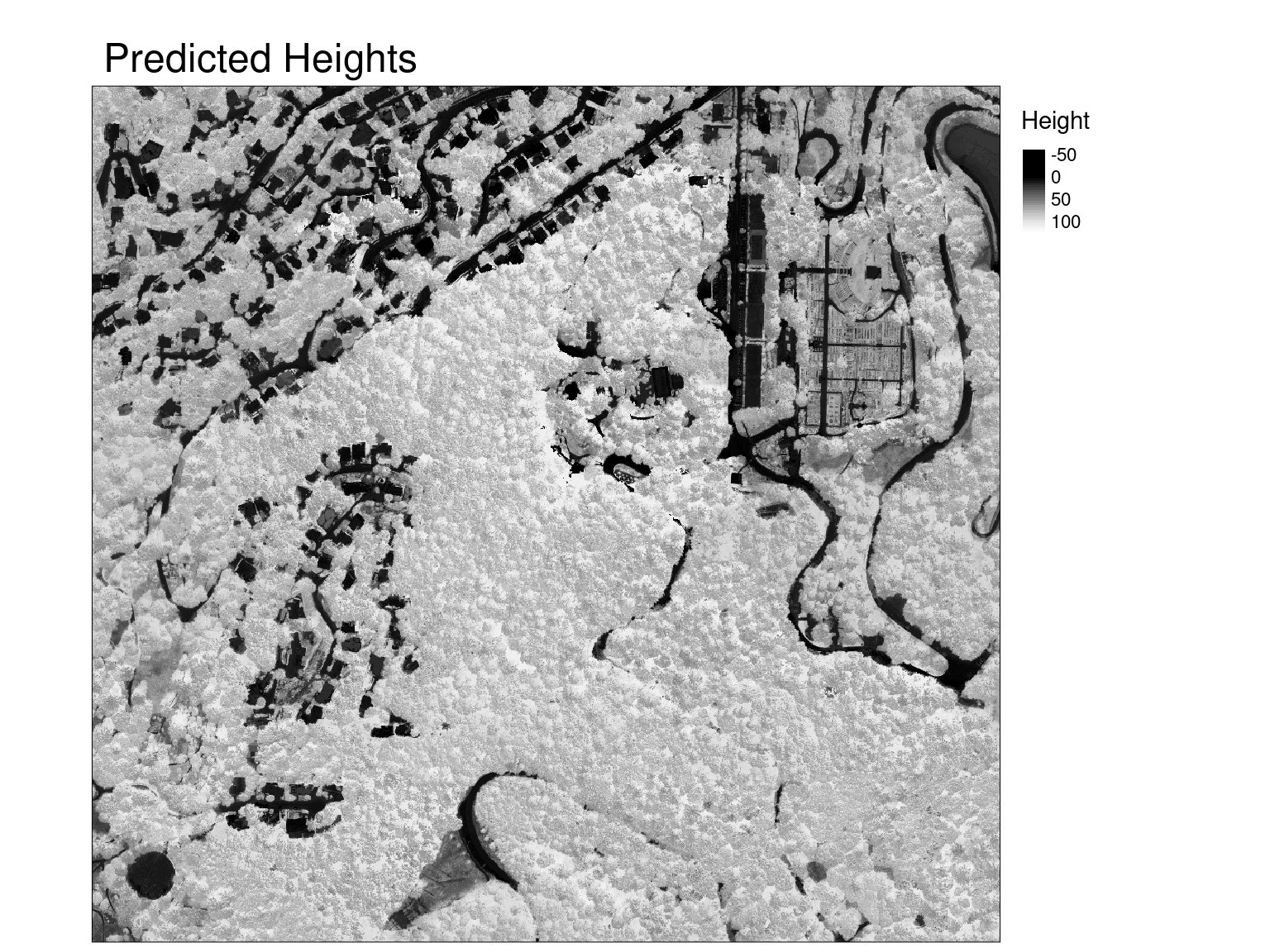
So… what are we looking at?
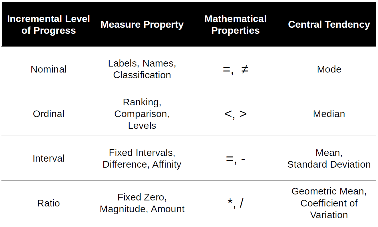
Steven’s Level of Measurement
NO
Steven’sStevens’ Level of Measurement
Nominal
- Labels or names; e.g. land use categories or soil types
Ordinal
- Ranked categories; e.g. flood risk
Interval
- Categories have fixed, equal units; e.g. Celsius or year
Ratio
- Have an inherent zero; e.g. distance, area, Kelvin
S.S. Stevens’ paper is ancient… 1946! https://marces.org/EDMS623/Stevens%20SS%20(1946)%20On%20the%20Theory%20of%20Scales%20of%20Measurement.pdf
Entity-Attribute Model
Commonly used in database design
Entity
- A readily identifiable object. It is independent and can be uniquely identified
- Tables and/or Rows
Attribute
- Characteristics of entities
- Columns
Wait a moment…
… it’s ‘tidy’!
Those of you with database experience will recognize this.
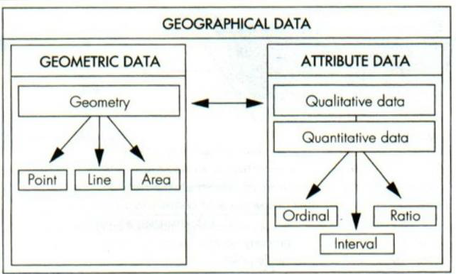
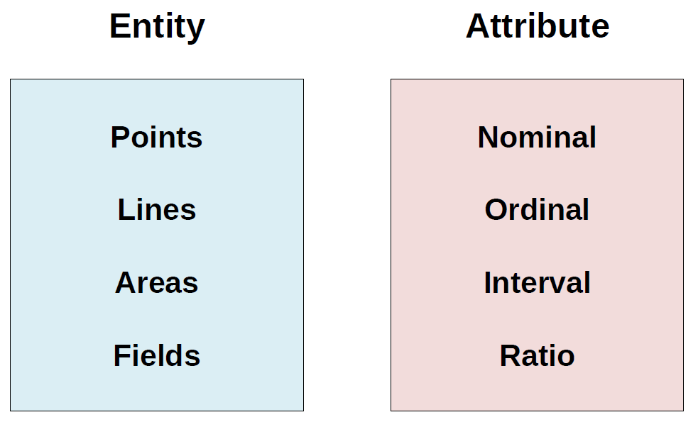
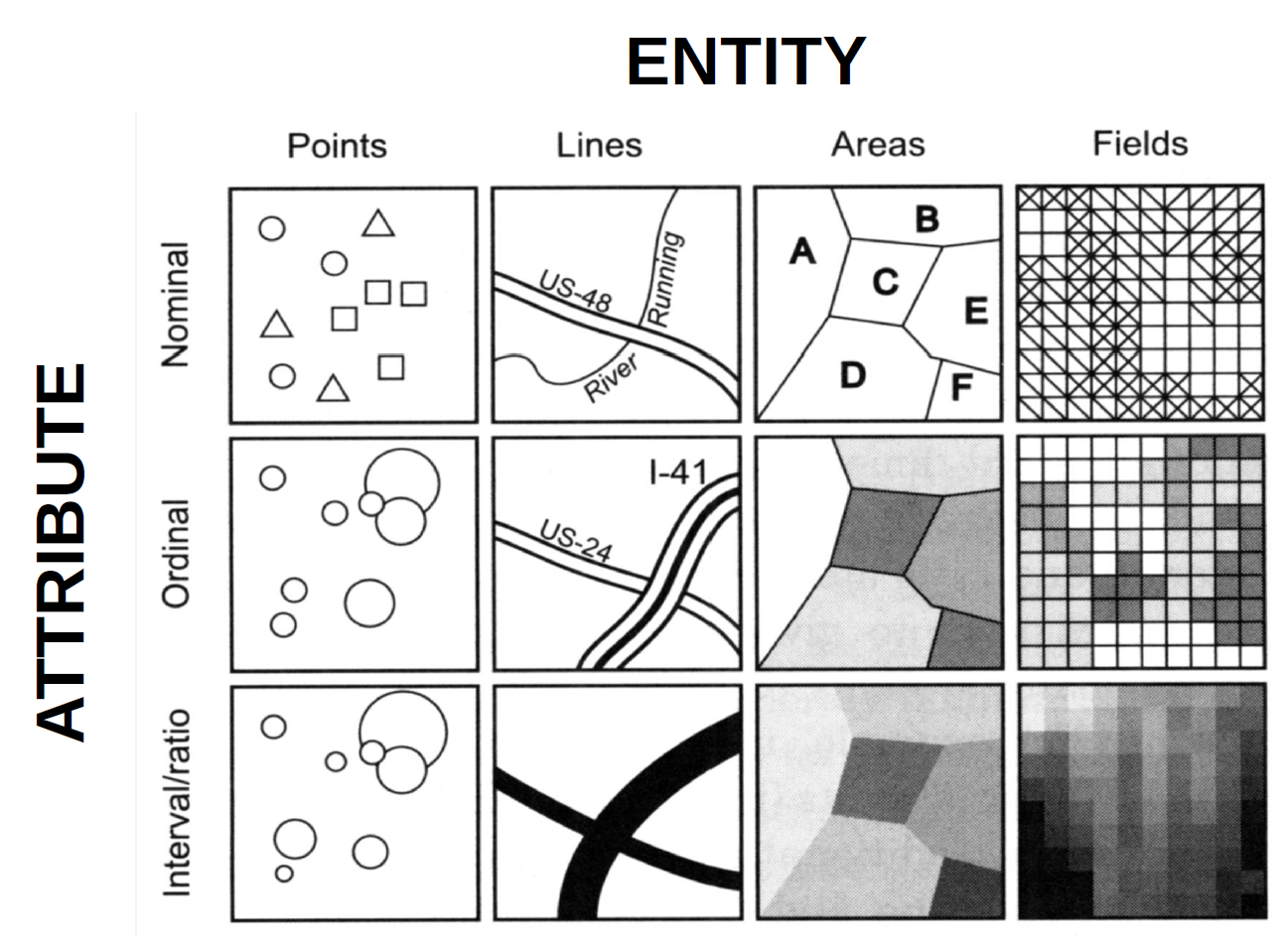
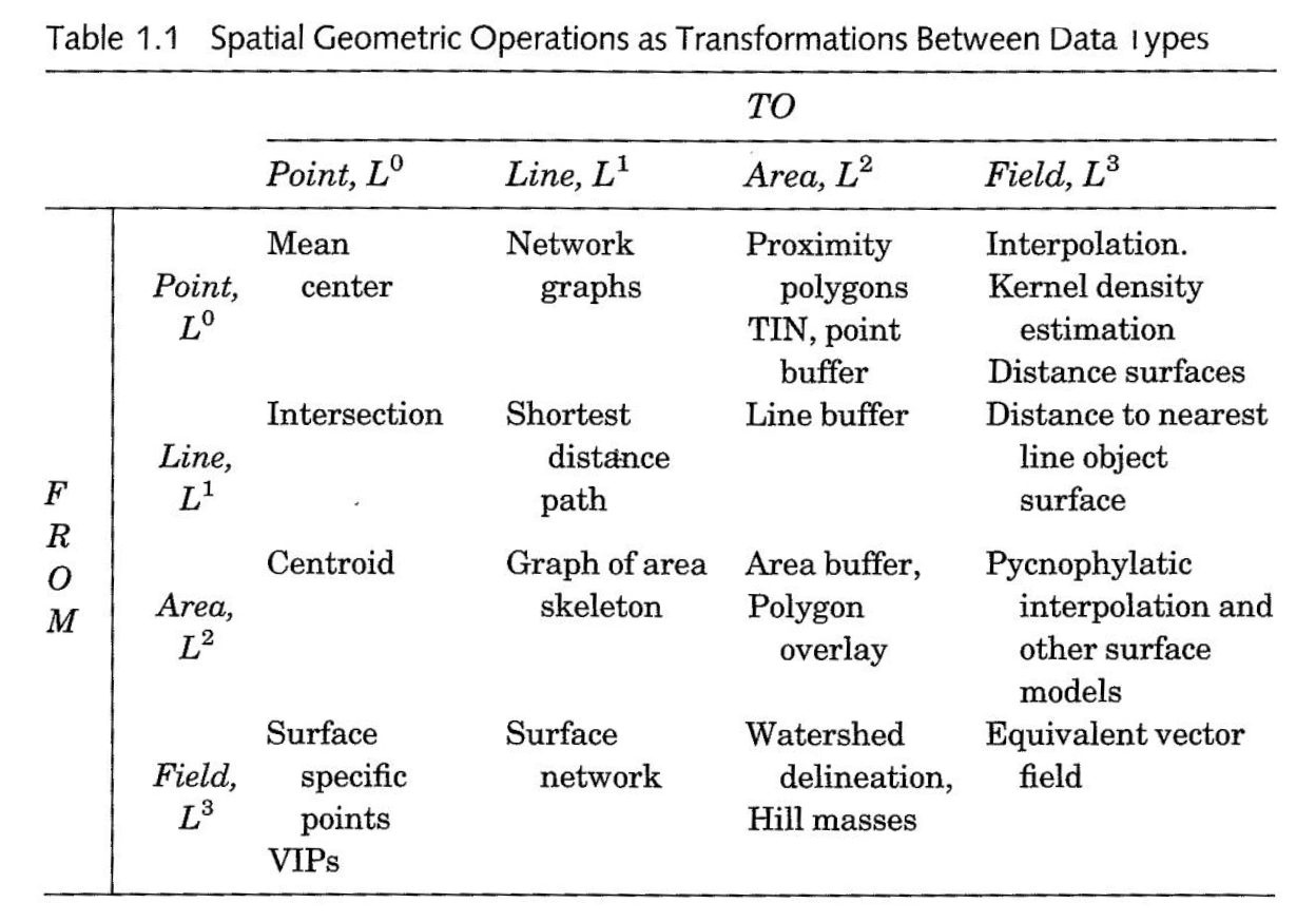
Most of the legwork in spatial analysis is battling the entity-attribute model:
- data formatting
- data transformation
- data munging
- geoenrichment (more on this week 8!)
Form of Data Influences Results
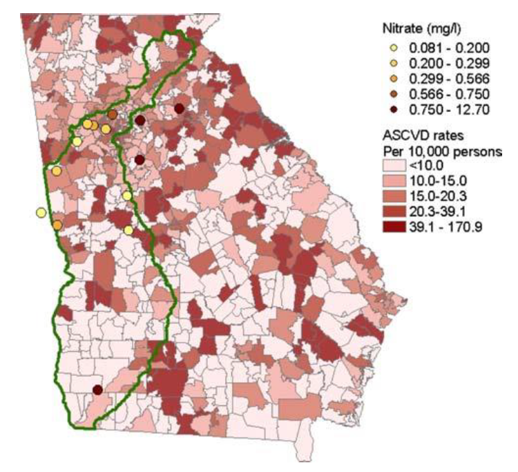
Young, and Gotway. 2007. “Linking spatial data from different sources: The effects of change of support.” Stochastic Environmental Research & Risk Assessment 21:589-600
Study assesses the interpolation results of risk based on ZIP polygon centroids and based on point samples.
Results are completely different, with addition of data
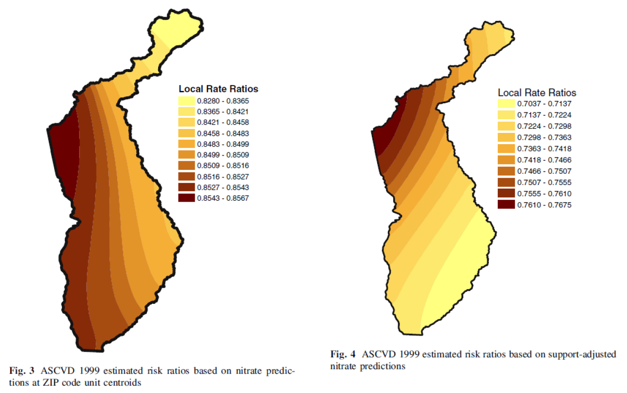
Young, and Gotway. 2007. “Linking spatial data from different sources: The effects of change of support.” Stochastic Environmental Research & Risk Assessment 21:589-600
Some Issues
Entity-attribute model is a simplification
- Reductive representation (e.g. county ID)
- Scale dependent
- Conversion between data types
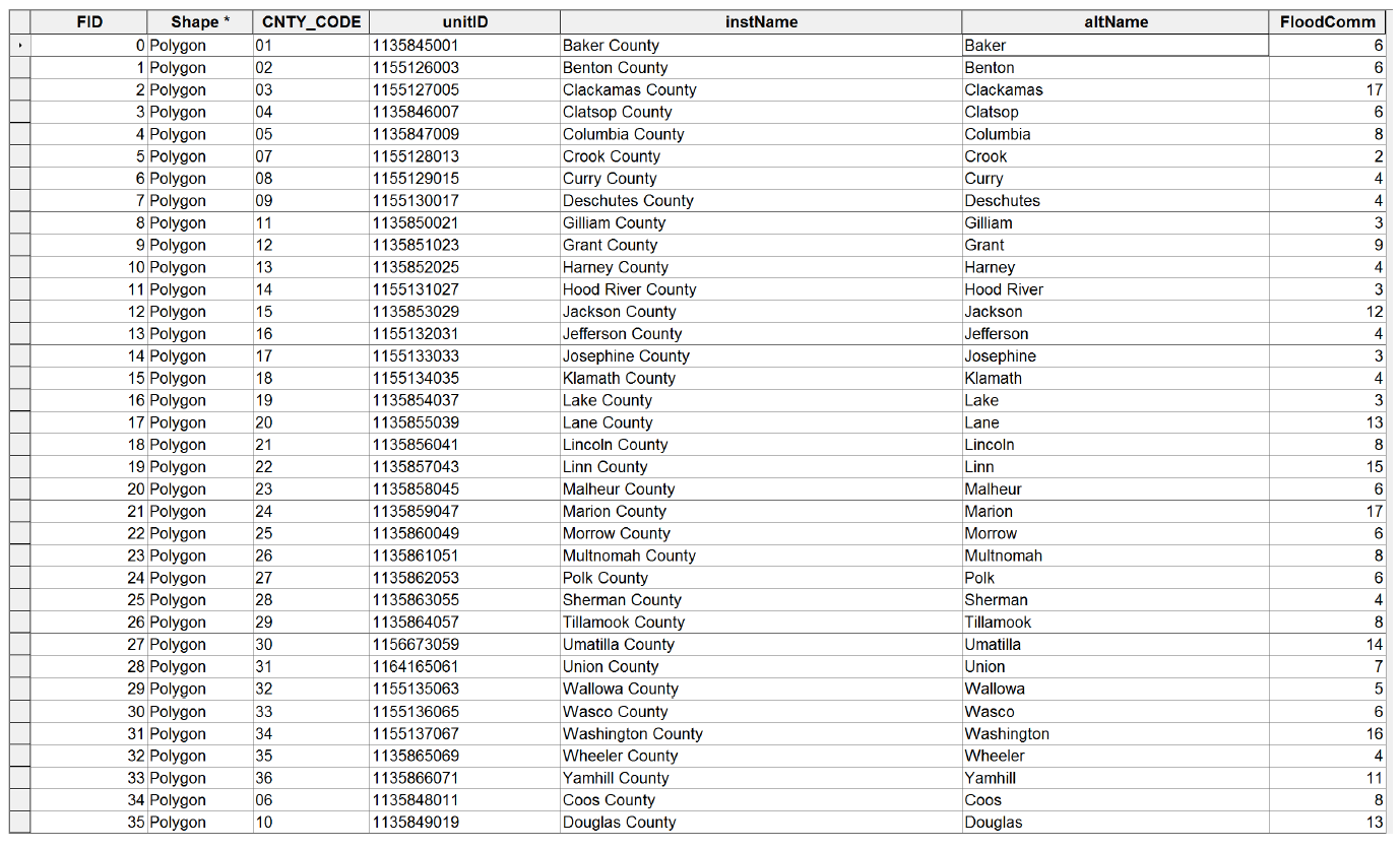
CNTY_CODE 26 … Multnomah
CNTY_CODE 09 … Deschutes (Rivi`re des Chutes)
Recommended Required Reading
( … down the rabbit hole … )

Bian, L. (2007). Object-Oriented Representation of Environmental Phenomena: Is Everything Best Represented as an Object? Annals of the Association of American Geographers, 97(2), 267-281. https://doi.org/10.1111/j.1467-8306.2007.00535.x
GIS & Spatial Analysis
- GIS usually claims to offer spatial analysis … but this doesn’t mean statistical spatial analysis
- Spatial data manipulation is readily available (buffer, overlay, spatial join)
- GIS has increased the need for spatial analysis, and lends some support
Spatial Analysis
Spatial Analysis is concerned with investigating the patterns that arise as a result of processes that may be operating in space. Techniques and methods to enable the representation, description, measurement, comparison and generation of spatial patterns are central to the study of geographic information analysis.
O’Sullivan and Unwin, page 4
Why isn’t spatial analysis in GIS?
GIS is built around the entity-attribute model. Spatial analysis uses these data, and sees data as patterns that are the outcomes of processes. This is similar… but different than spatial data manipulation.
In short, I’m trying to make you think like a data analyst who can utilize spatial information and not a GIS analyst who knows some data analysis techniques (or worse, some buttons in ArcGIS)
Summary
- We usually distinguish spatial analysis from GIS operations and spatial modeling
- Spatial data in the entity-attribute model combines the entity with its attributes in various combinations
- … which has a many issues
- … and is always reductive (read Bian 2007!)
- Spatial analysis is still poorly supported by GIS, but it is improving.
For Next Week
DataCamp
Do some exercises! Do a bunch!
You could easily knock out several before Monday, and free yourself up later in the term (or just learn more).
Lab
There’s no lab, because we haven’t even really learned anything yet!
Don’t worry, we’re just laying a sturdy foundation and will dive in next week.
Bian (2007)
I consider this one of the most definitive papers in our field. But it is dry…