Problems with Spatial Data
GEOG 4/597: Advanced Spatial Quantitative
Analysis, Winter 2023
Jackson Voelkel | Portland State
University
plot(mod,3)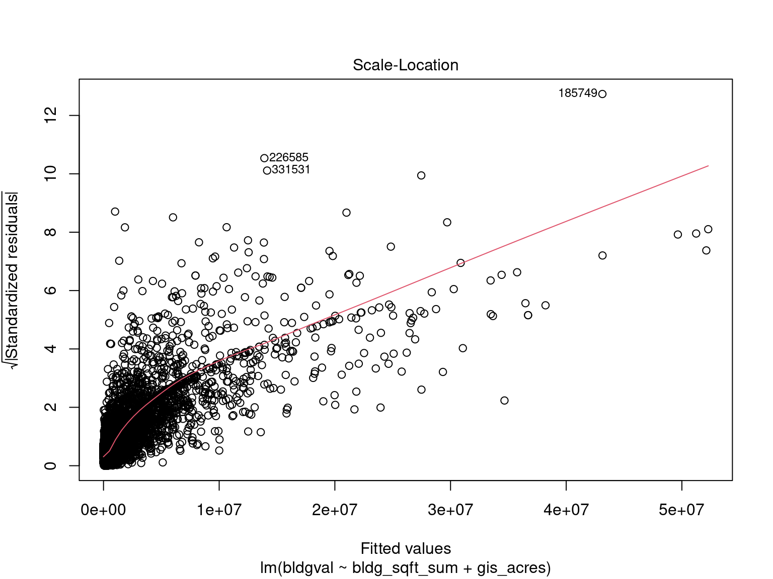
“As building value (bldgval) increases, so does
our error.” or “Our model is better at predicting home values for
less expensive homes”
Spatial Autocorrelation
Actual Population
->
Random Population
https://mgimond.github.io/Spatial/spatial-autocorrelation.html
Spatial Autocorrelation
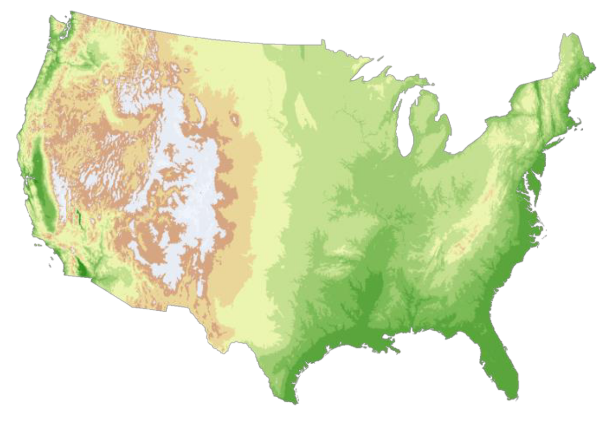
Actual Elevation
->
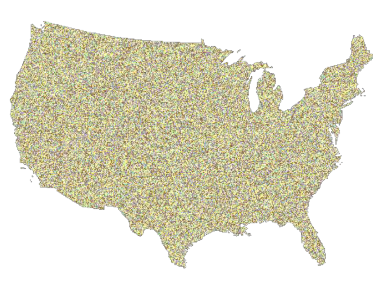
Random Elevation
https://mgimond.github.io/Spatial/spatial-autocorrelation.html
First Order Variation
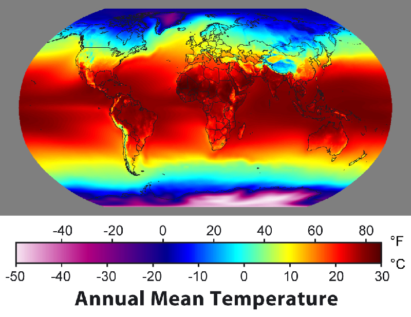
https://en.wikipedia.org/wiki/File:Annual_Average_Temperature_Map.jpg
So what?
1. We can take note of this, and include it in
our analysis considerations…
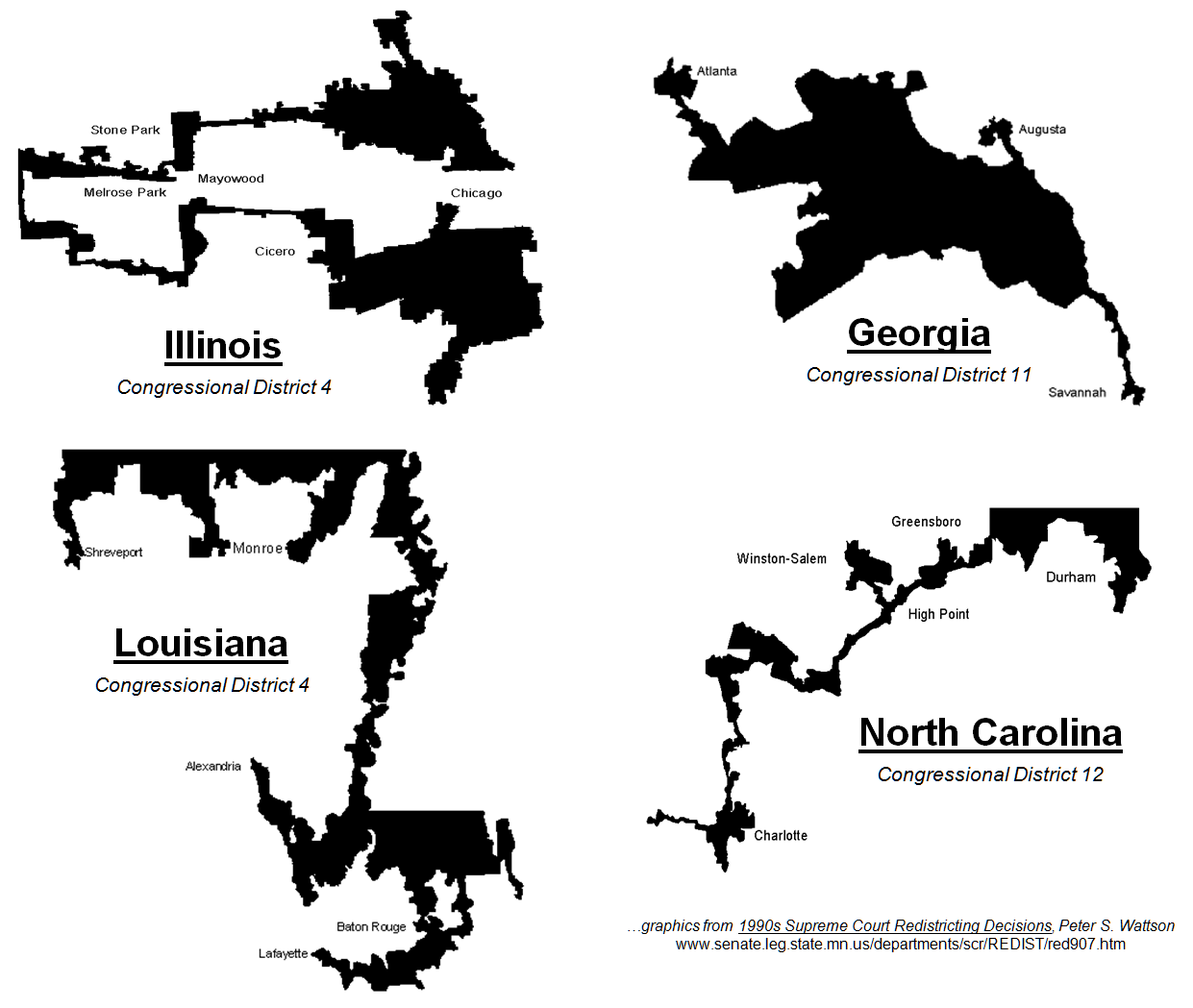
2. … or
we can use it for voter suppression!

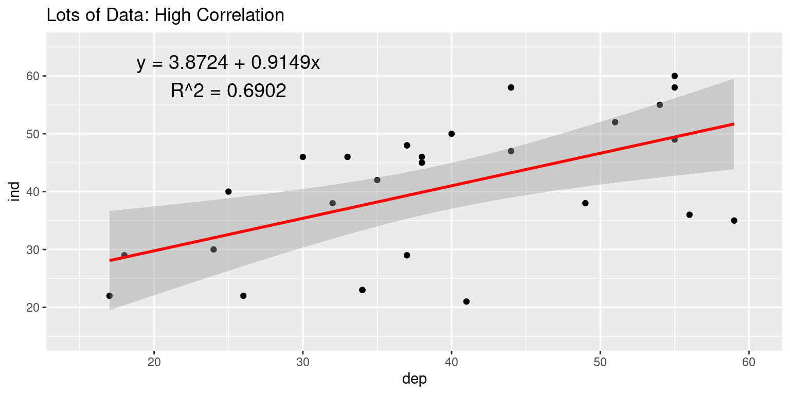
Modifiable Areal Unit Problem (MAUP)
Our choice of spatial reference frame is itself a significant determinant of the statistical and other patterns we observe.
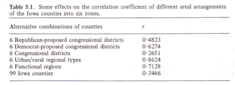
x = % of population over 62; y= % vote
for Republican congressional candidates (1968)
Openshaw, S. and P.J. Taylor. 1979. “A million or so correlation coefficients: Three experiments on the modifiable areal unit problem.” Pp. 127-144 in Statistical Methods in the Spatial Sciences, edited by N. Wrigley. London: Pion.
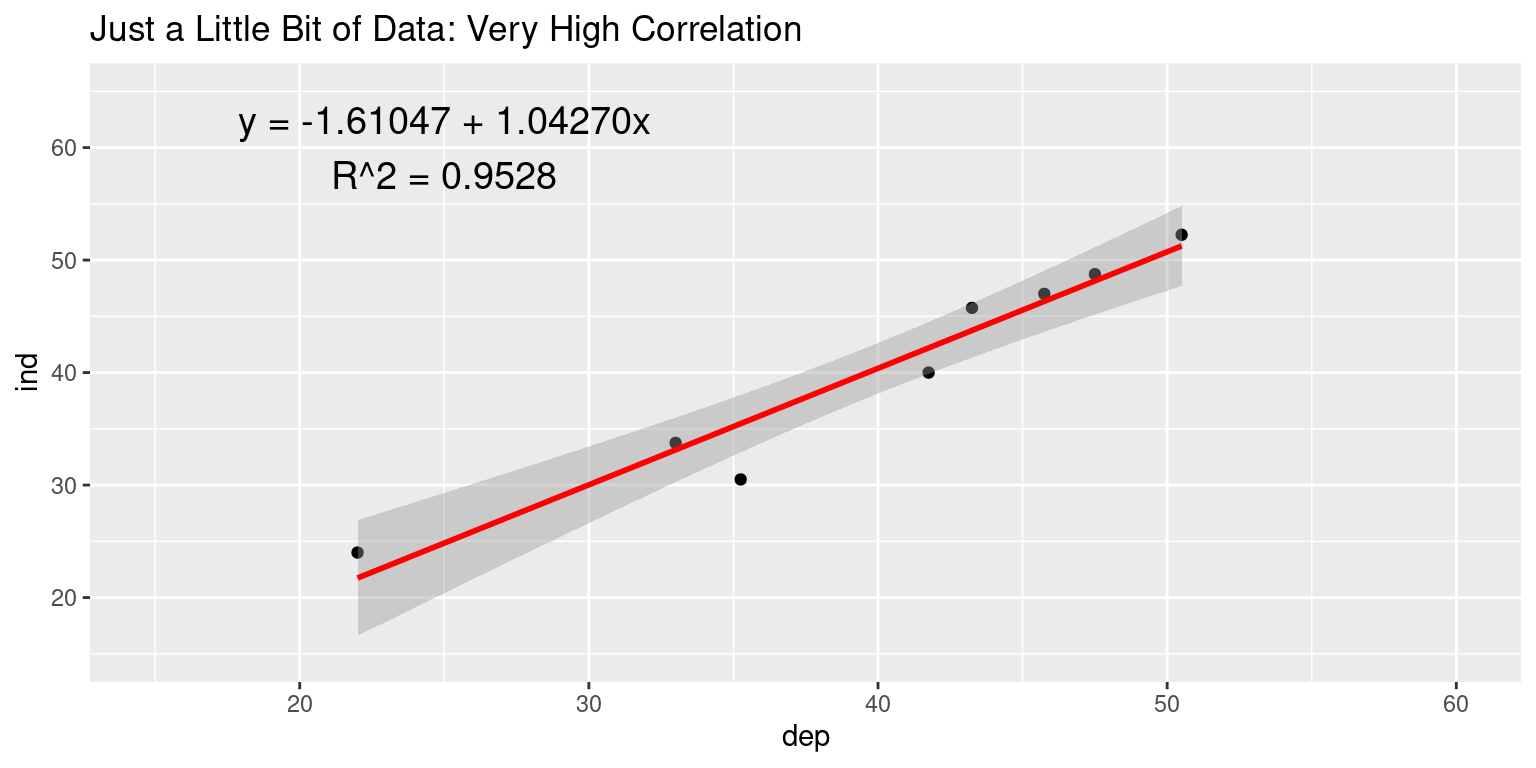
Modifiable Areal Unit Problem (MAUP)
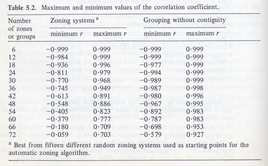
Openshaw, S. and P.J. Taylor. 1979. “A million or so correlation coefficients: Three experiments on the modifiable areal unit problem.” Pp. 127-144 in Statistical Methods in the Spatial Sciences, edited by N. Wrigley. London: Pion.
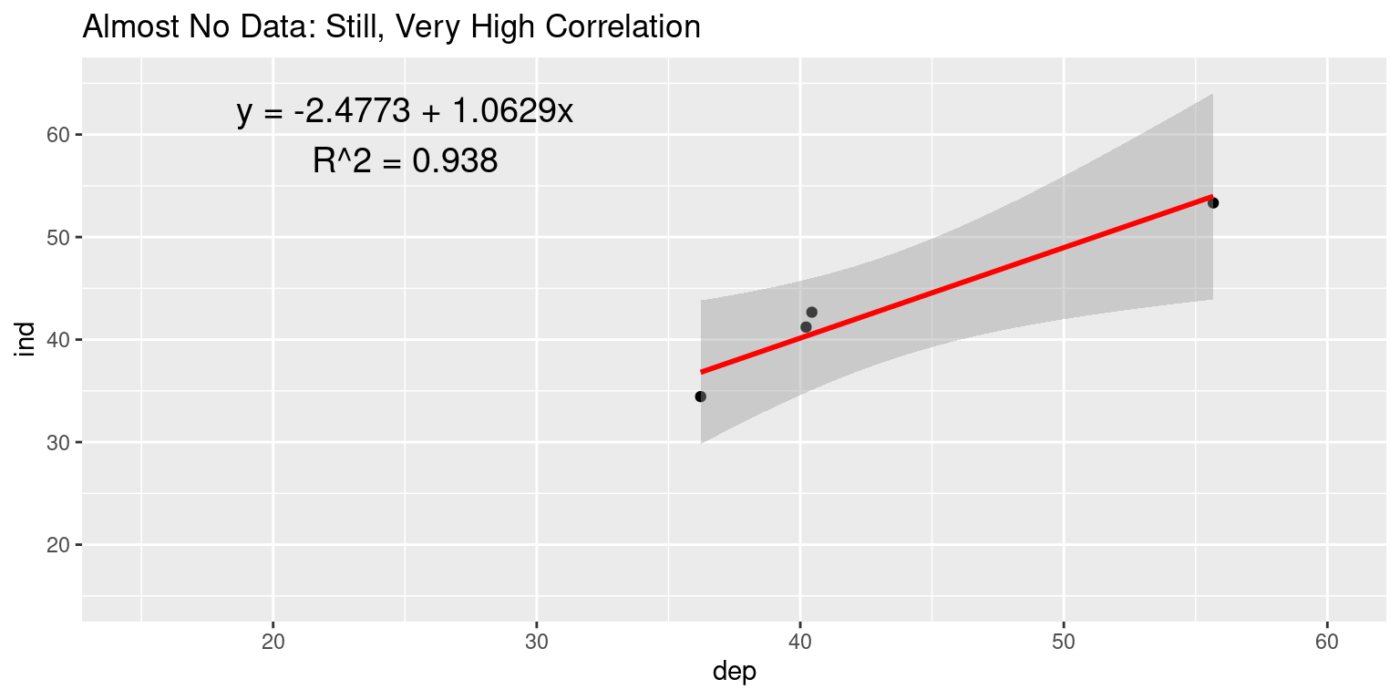
Modifiable Areal Unit Problem (MAUP)
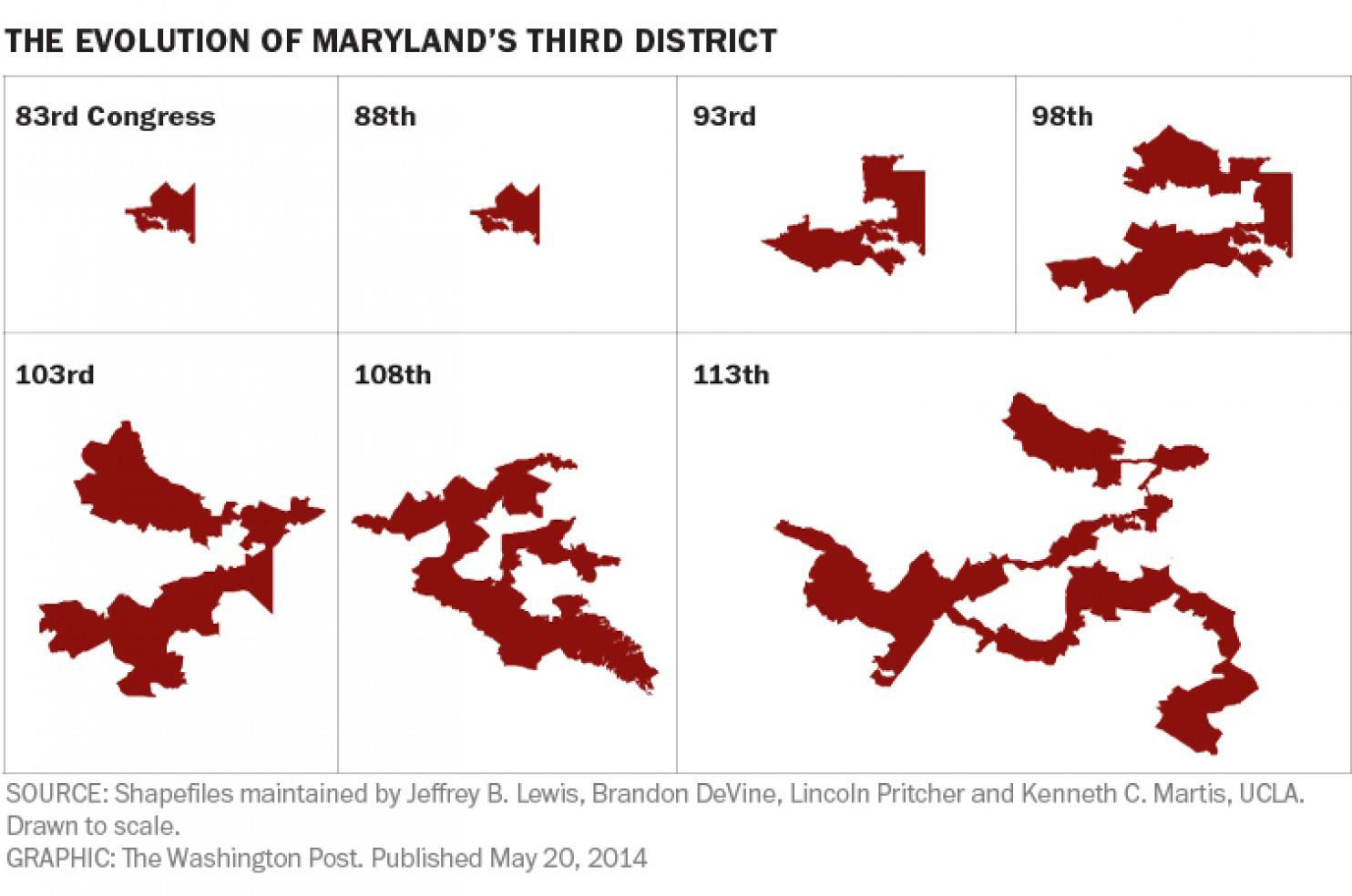
Modifiable Areal Unit Problem (MAUP)
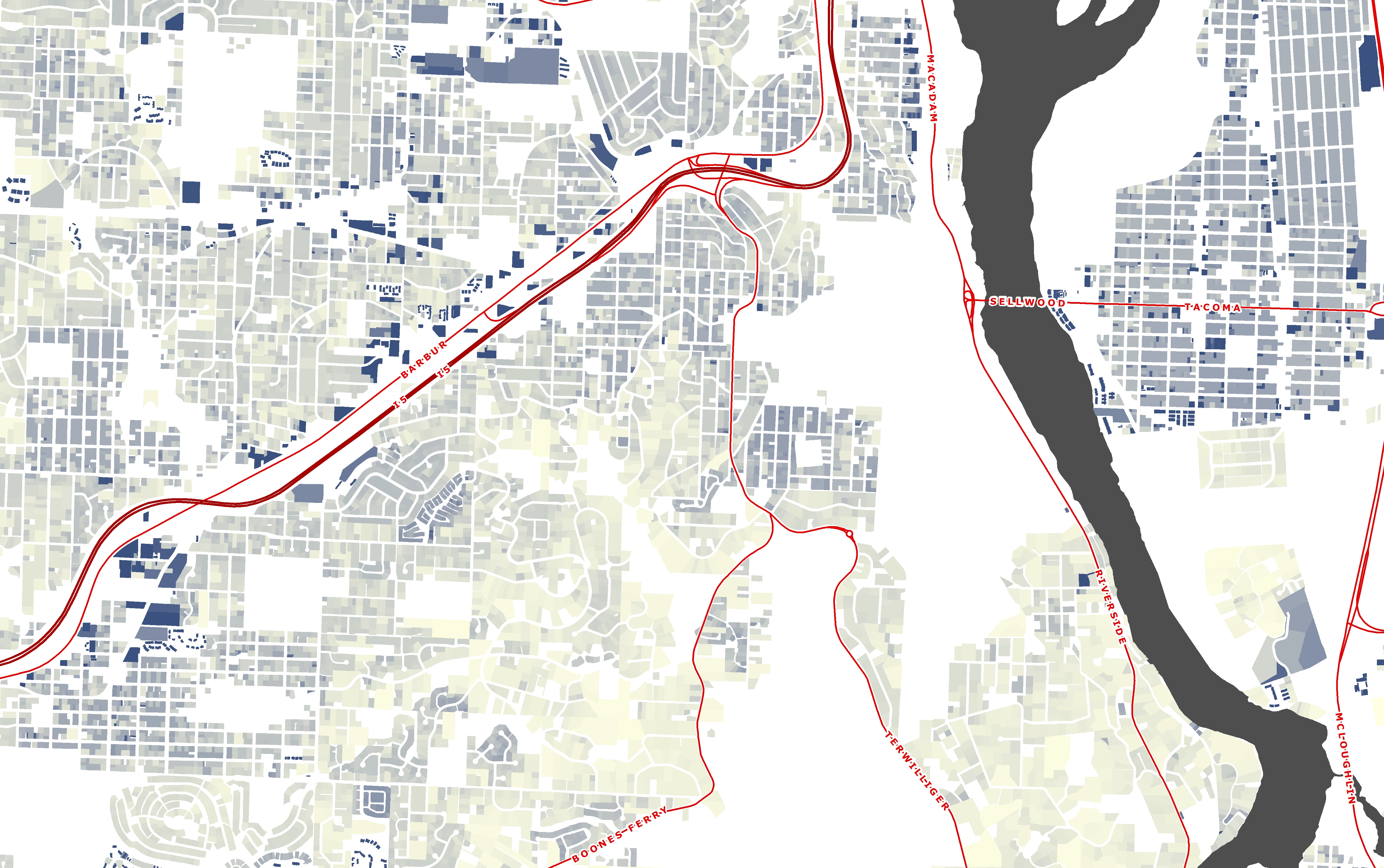
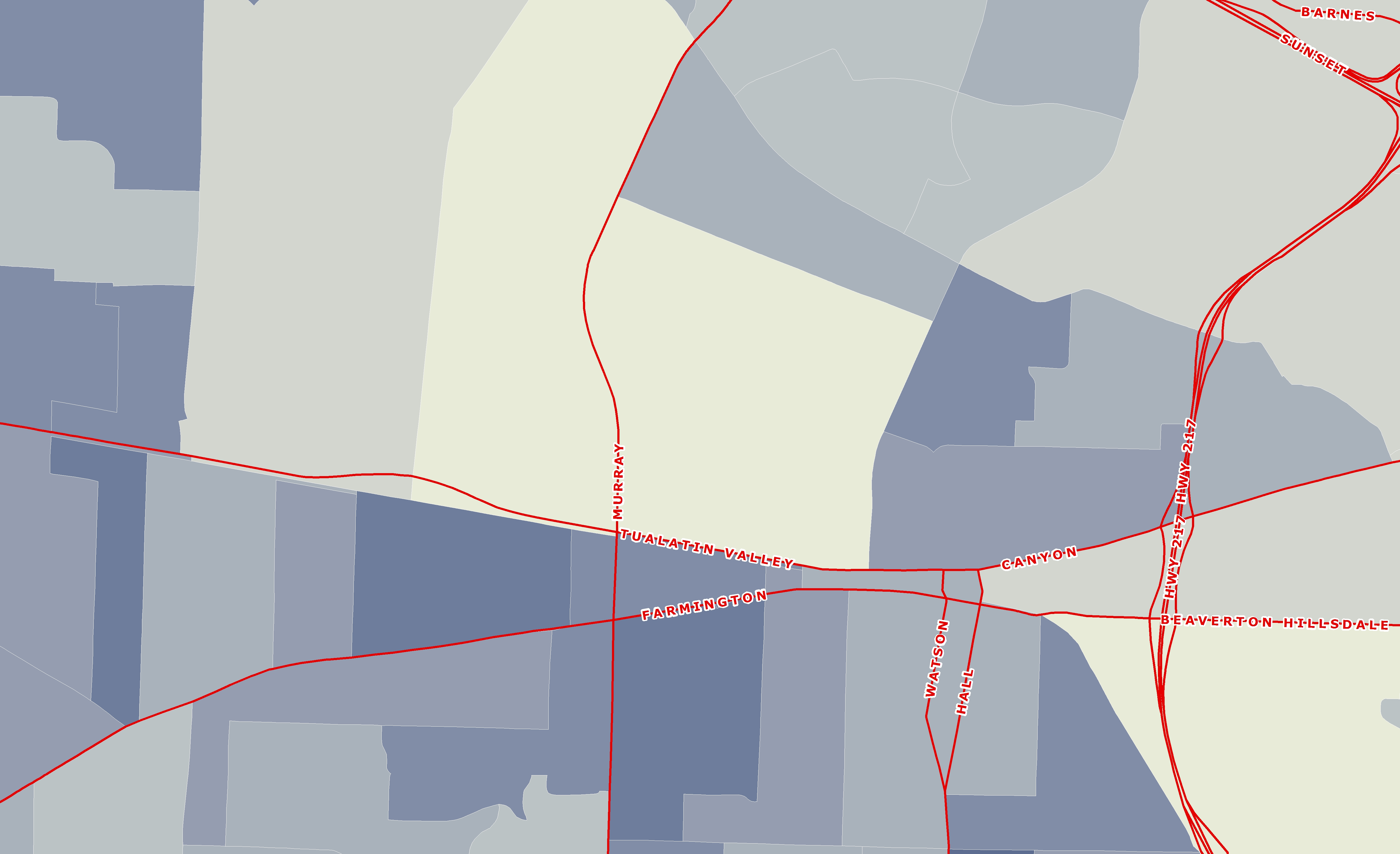
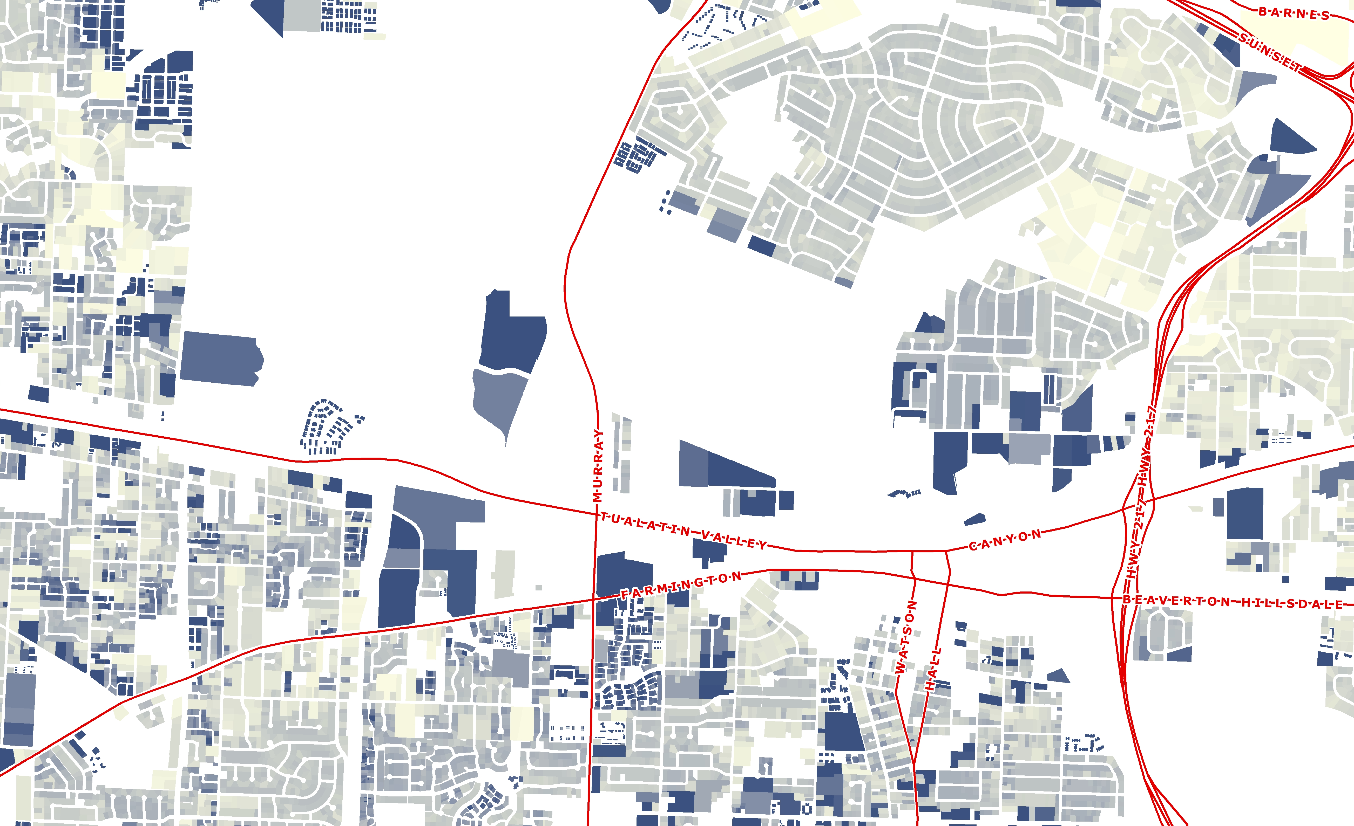
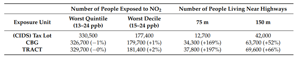
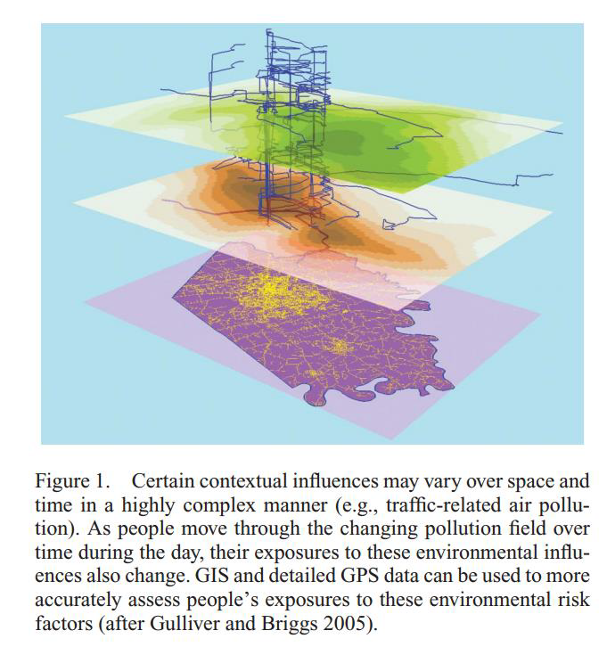
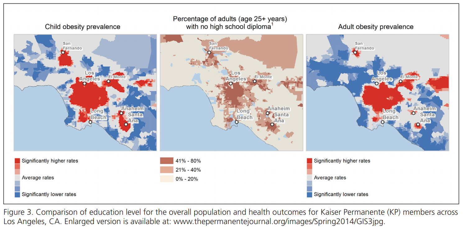
Assessing Exposure
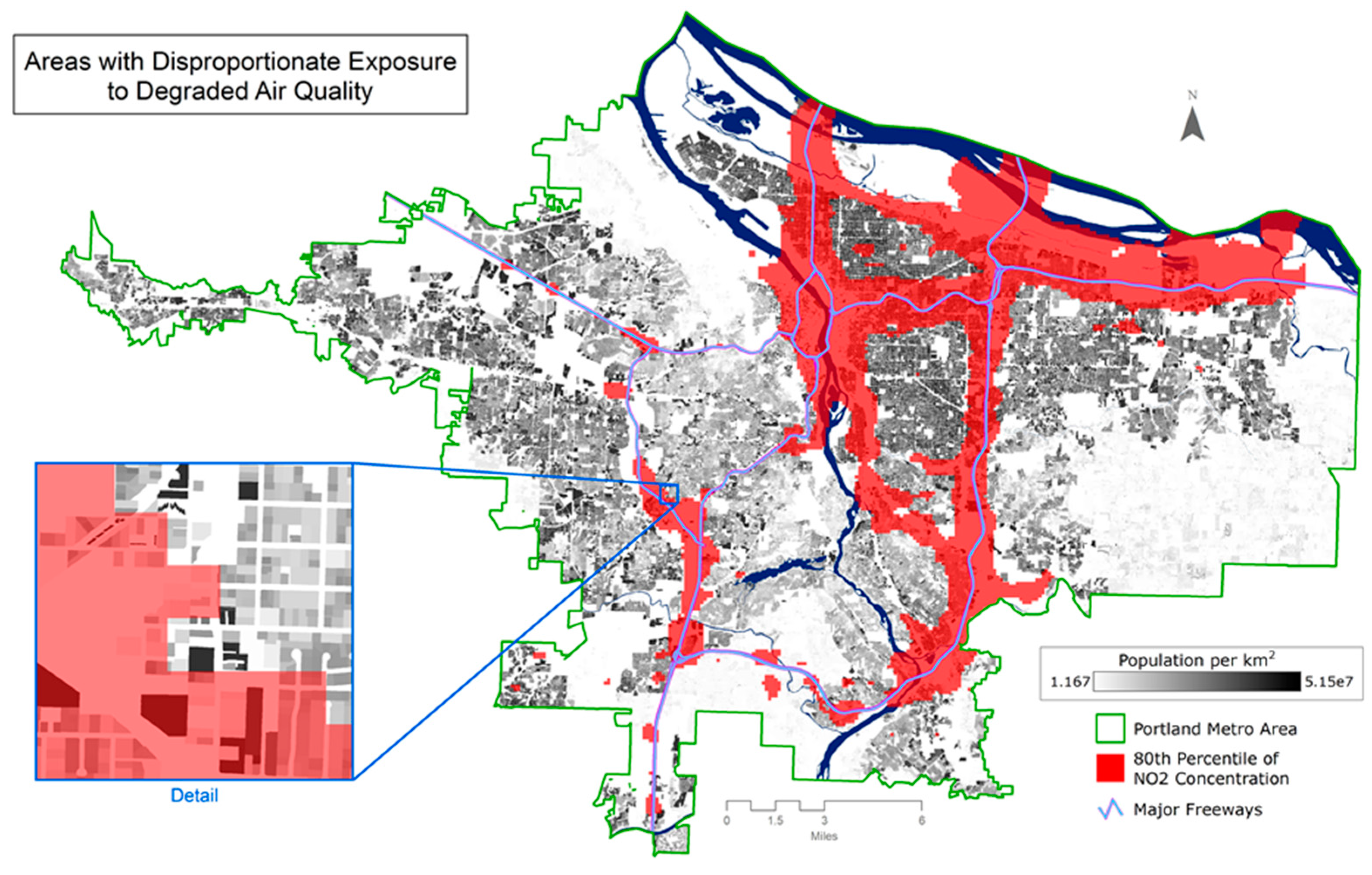
Assessing Exposure
Comparing Dasymetric population data to standard census geometries:
Dependent
| 87 | 95 | 72 | 37 | 44 | 24 |
| 40 | 55 | 55 | 38 | 88 | 34 |
| 41 | 30 | 26 | 35 | 38 | 24 |
| 14 | 56 | 37 | 34 | 8 | 18 |
| 49 | 44 | 51 | 67 | 17 | 37 |
| 55 | 25 | 33 | 32 | 59 | 54 |
Independent
| 72 | 75 | 85 | 29 | 58 | 30 |
| 50 | 60 | 49 | 46 | 84 | 23 |
| 21 | 46 | 22 | 42 | 45 | 14 |
| 19 | 36 | 48 | 23 | 8 | 29 |
| 38 | 47 | 52 | 52 | 22 | 48 |
| 58 | 40 | 46 | 38 | 35 | 55 |
Dependent
| 69.25 | 50.5 | 47.5 |
| 35.25 | 33 | 22 |
| 43.25 | 45.75 | 41.75 |
Independent
| 64.25 | 52.25 | 48.75 |
| 30.5 | 33.75 | 24 |
| 45.75 | 47 | 40 |
Dependent
| 55.67 | 40.22 |
| 40.44 | 36.22 |
Independent
| 53.33 | 41.22 |
| 42.67 | 34.44 |
cnty %>% tm_shape() +
  tm_polygons(col='estimate', title="MHI", palette = "YlGnBu",
              border.col = 'white',lwd=0.5) +
  tm_layout(main.title = "Median Household Income: County")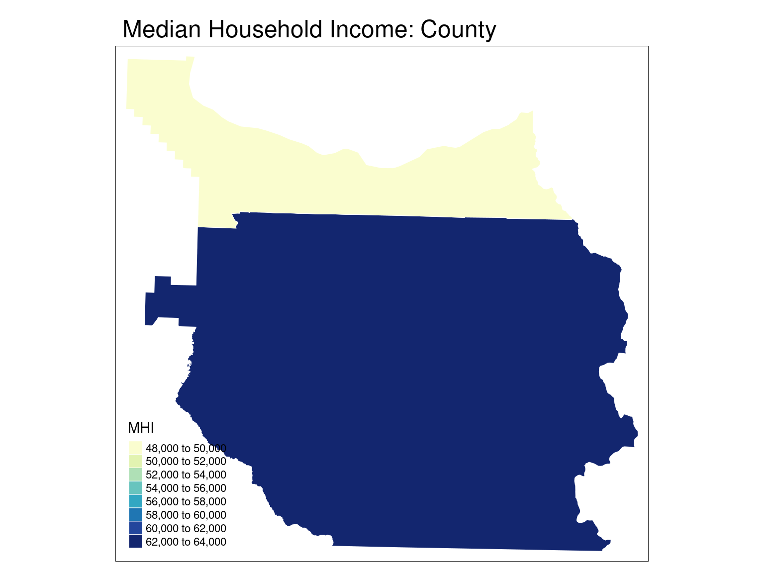
trct %>% tm_shape() +
  tm_polygons(col='estimate', title="MHI", palette = "YlGnBu",
              border.col = 'white',lwd=0.5) +
  tm_layout(main.title = "Median Household Income: Tract")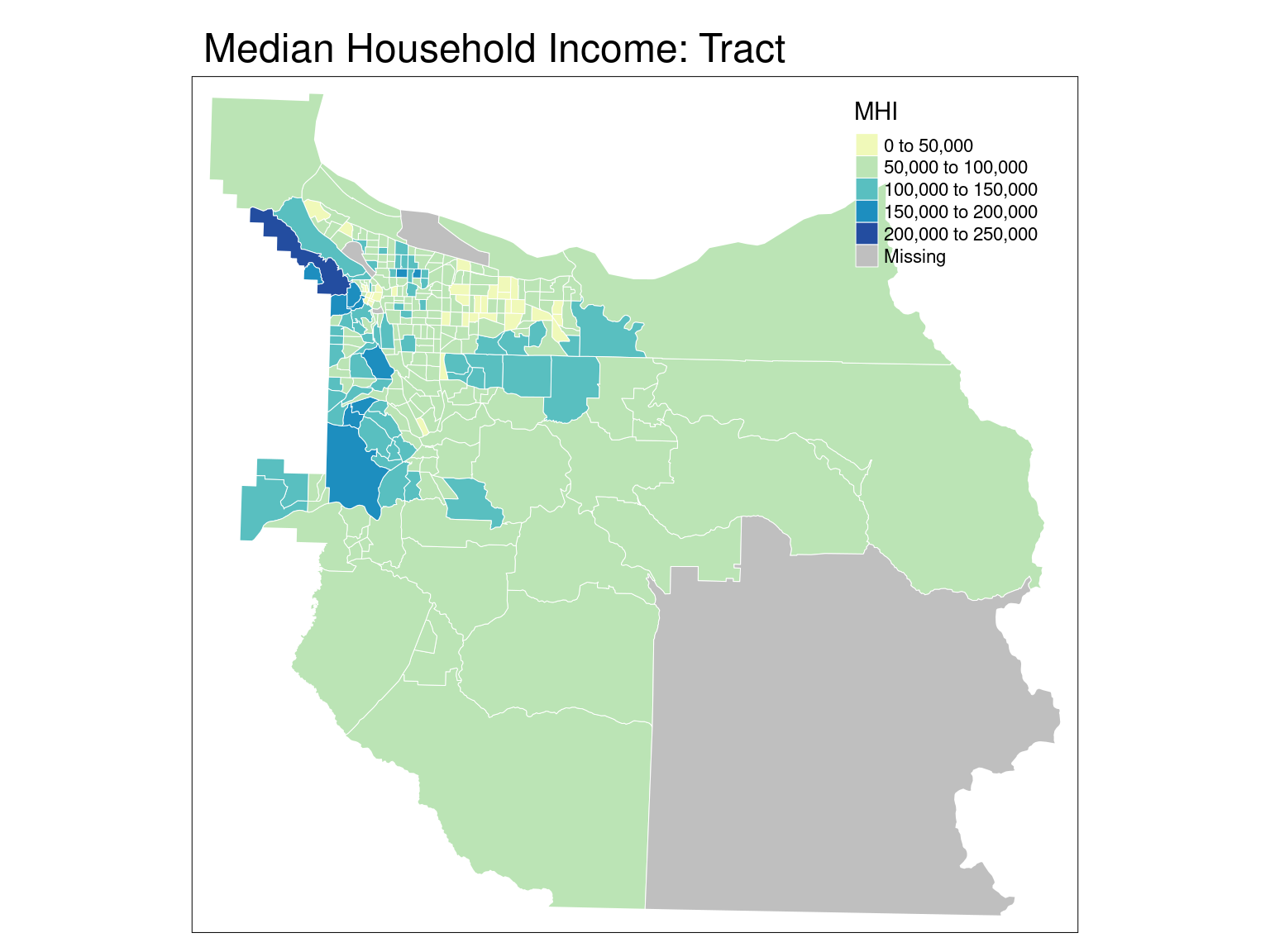
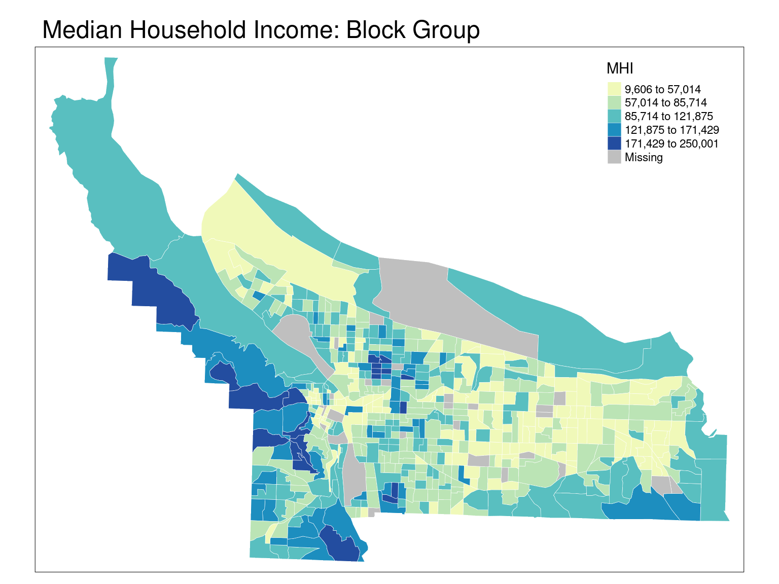
bg %>% tm_shape() +
  tm_polygons(col='estimate', title="MHI", palette = "YlGnBu",
              border.col = 'white',lwd=0.3, style="jenks") +
  tm_layout(main.title = "Median Household Income: Block Group")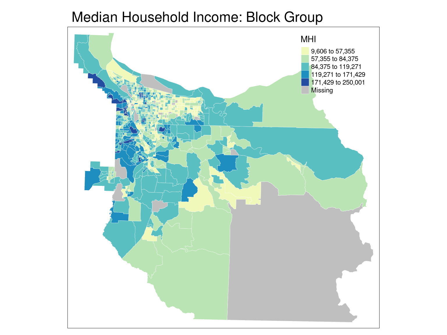
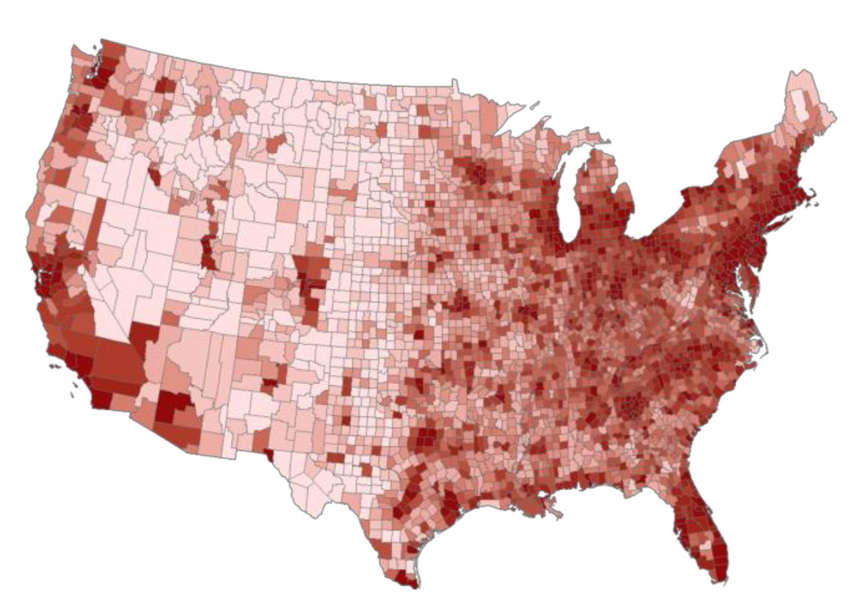
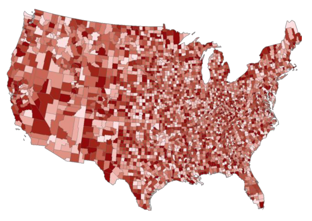
cnty %>% tm_shape() +
  tm_polygons(col='pct_hl', title="% of Pop.", palette = "YlGnBu",
              border.col = 'white', lwd=0.5) +
  tm_layout(main.title = "Hispanic or Latino: County")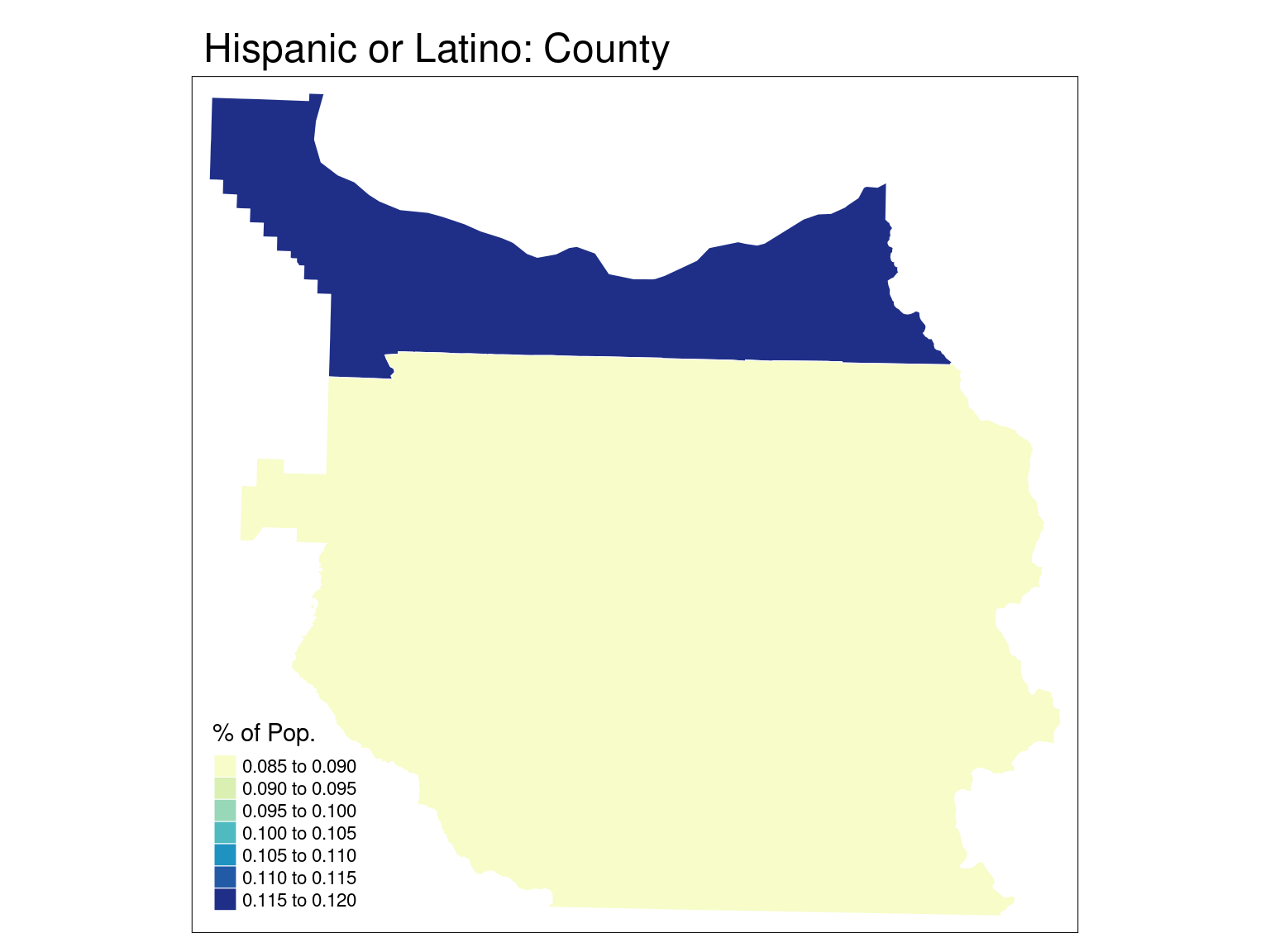
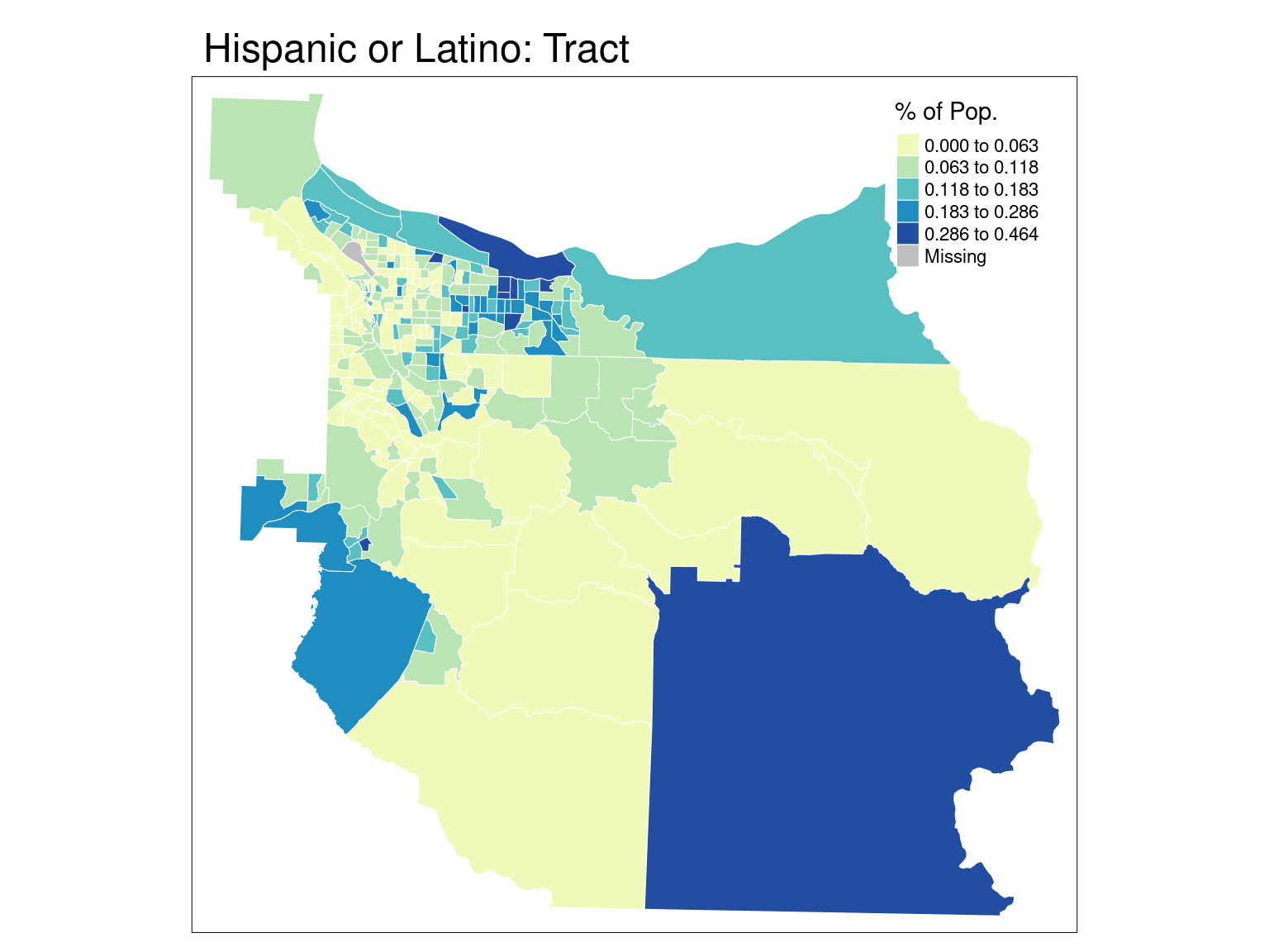
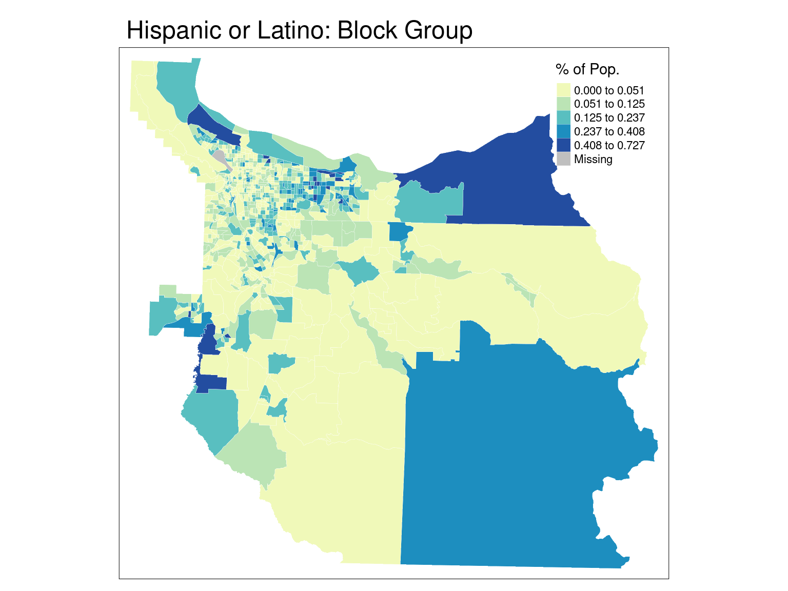
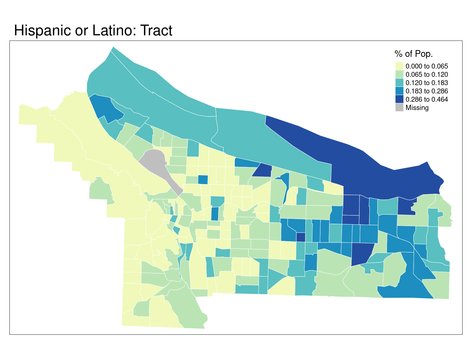
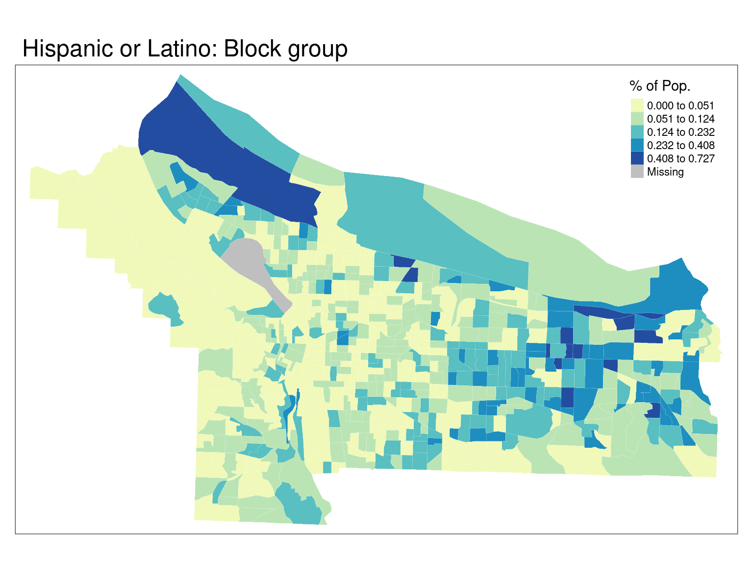
Scale: Census Geographies
Scale and Resolution
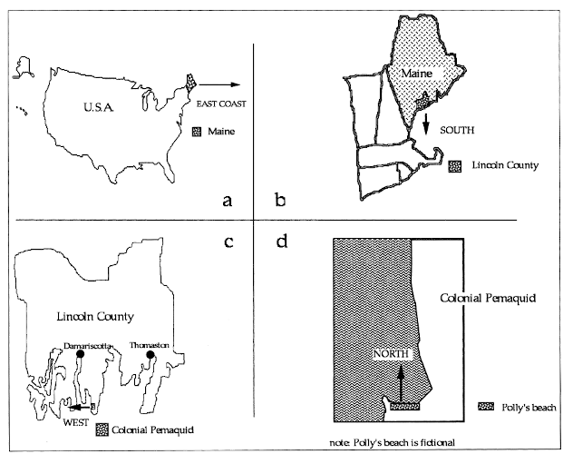
Kwan, Mei-Po. 2012. “How GIS can help address the uncertain geographic context problem in social science research.” Annals of GIS 18:245-255.

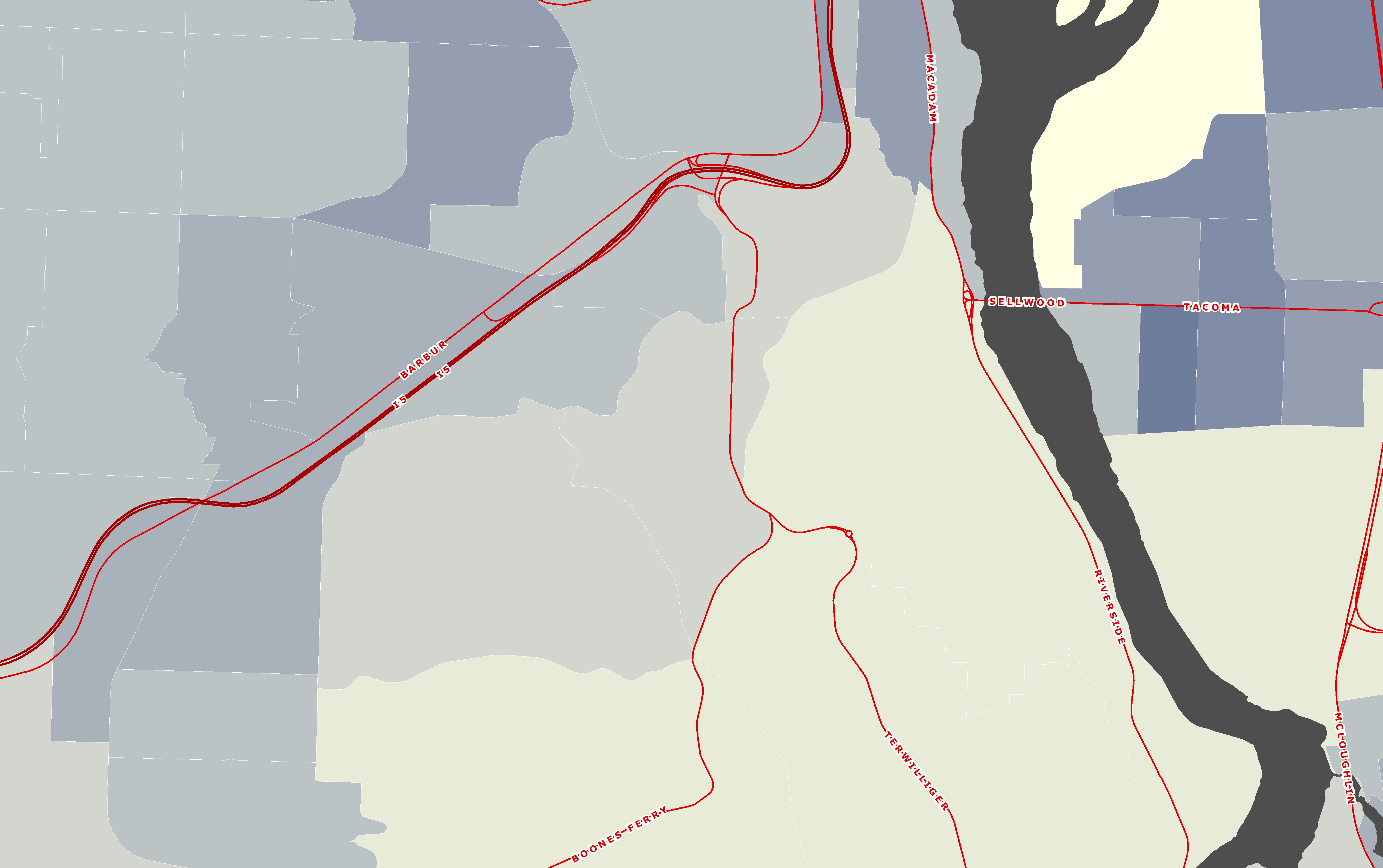
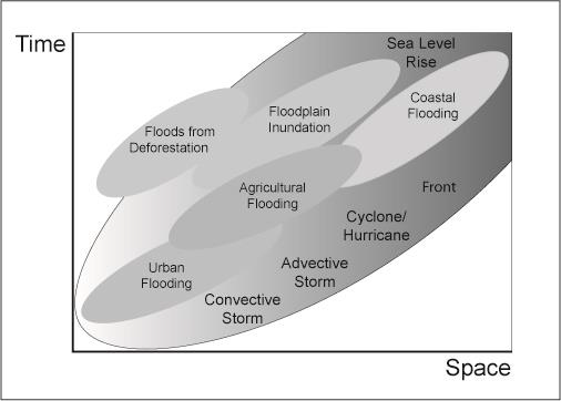
Non-uniformity of Space
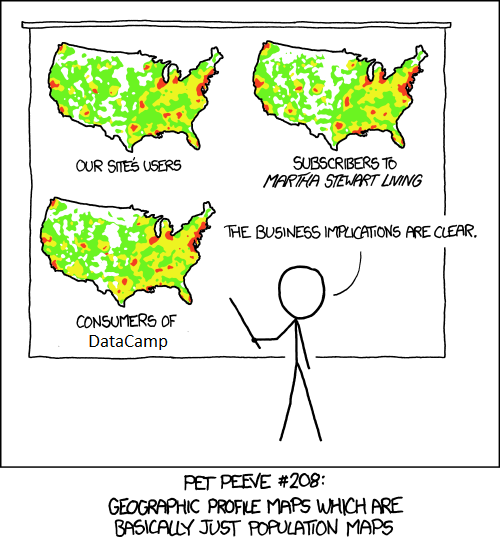
Source: XKCD
Non-uniformity of Space
Non-uniformity of Space
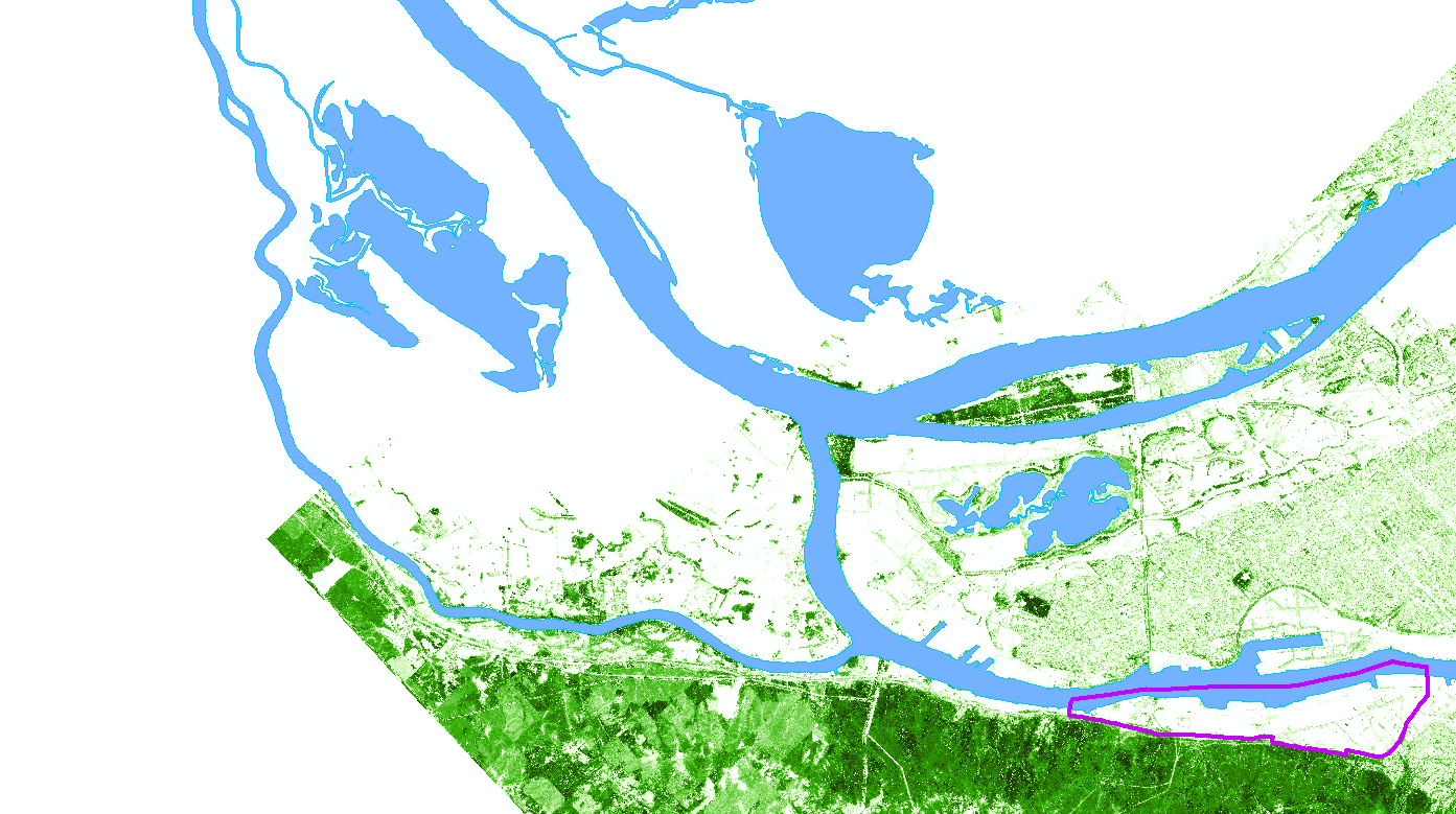
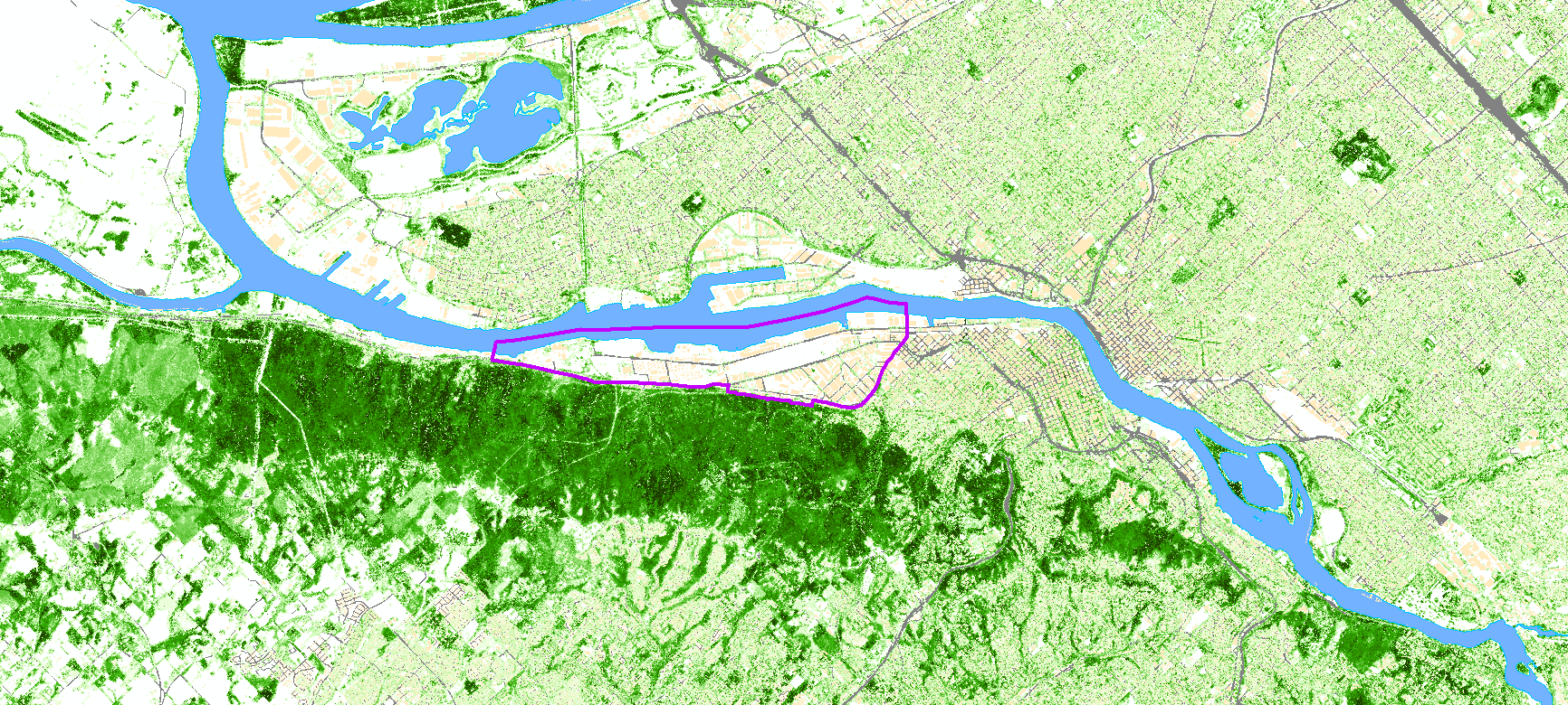
Model NOx for an Industirial Area
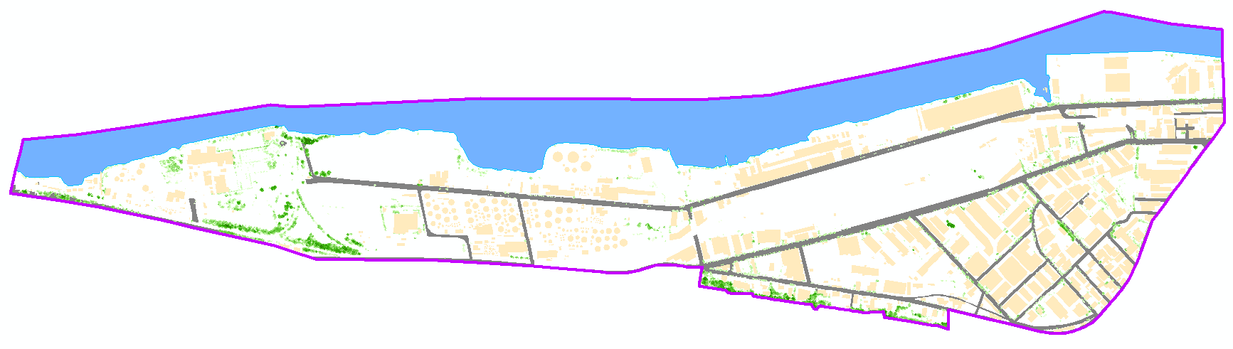
Model NOx for an Industirial Area
Model NOx for an Industirial Area
Model NOx for an Industirial Area
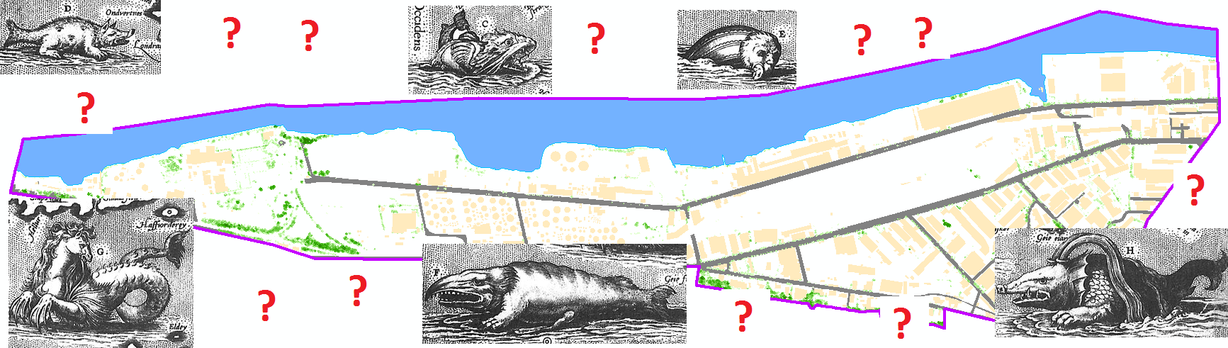
Maybe our initial model has some issues…
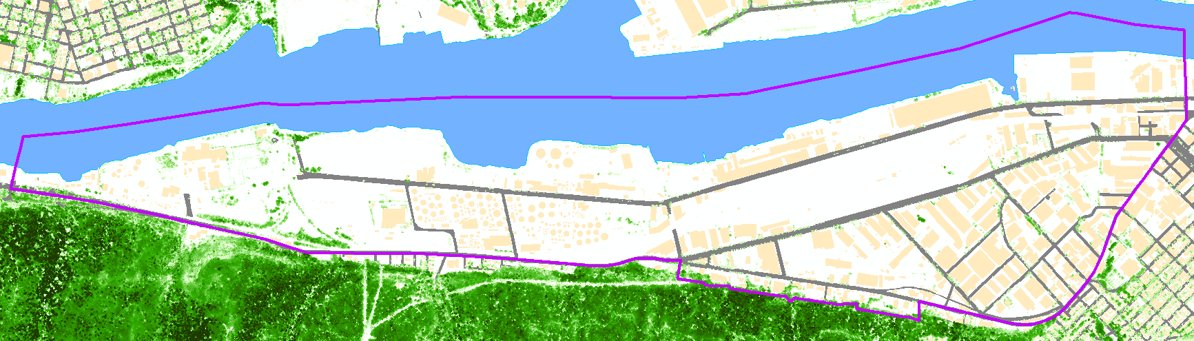
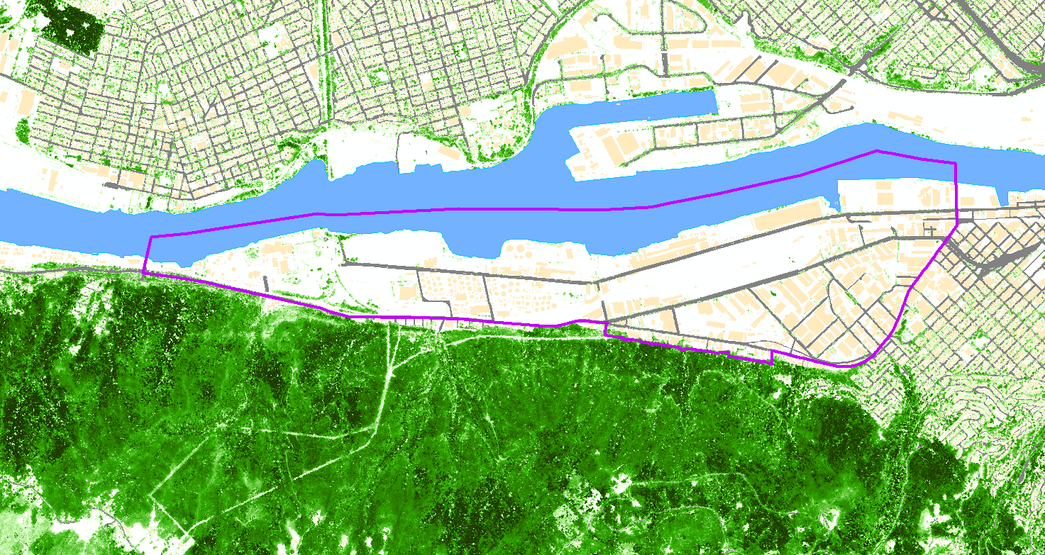
What scale best fixes edge effects?
- It depends!

Edge effects via data limitations