Point Pattern Analysis I


GEOG 4/597: Advanced Spatial Quantitative Analysis, Winter 2023

Jackson Voelkel   |   Portland State University

Overview


  • Definition of point pattern
  • Framework for spatial analysis
  • Two ways of measuring: density-based, distance-based

Point Pattern

Definition


Point patterns, where the only data are the locations of a set of point objects


  • The simplest possible spatial data (though not simple to analyze)
  • A set of events in a study area
  • An event is a relevant observation at some point location

Location is the Only Data

# Warning: Some wild code happening here!
suppressPackageStartupMessages(require(dplyr))
suppressPackageStartupMessages(require(rvest))
suppressPackageStartupMessages(require(sf))
suppressPackageStartupMessages(require(tmap))
tmap_mode('view')

url <- "https://en.wikipedia.org/wiki/List_of_hydroelectric_power_stations_in_the_United_States"
dams <- url %>% read_html() %>% 
  html_node(xpath = '//*[@id="mw-content-text"]/div[1]/table[1]') %>% 
  html_table(trim = T) %>% 
  mutate(
    y = Coordinates %>% 
          strsplit(" / |\\(") %>% 
          sapply('[',3) %>% 
          strsplit(";") %>% 
          sapply('[',1) %>% 
          trimws() %>% gsub("[^[:alnum:] \\.-]","",.) %>% as.numeric(),
    x = Coordinates %>% 
          strsplit(" / |\\(") %>% 
          sapply('[',3) %>% 
          strsplit(";") %>% 
          lapply('[',2) %>% 
          unlist %>% 
          trimws() %>% gsub("[^[:alnum:] \\.-]","",.) %>% as.numeric(),
    sus_output = `Capacity(MW)` %>% gsub(",","",.) %>% as.numeric
  ) %>% 
  dplyr::arrange(-sus_output) %>% 
  filter(!is.na(x),!is.na(y)) %>% 
  filter(!is.na(sus_output)) %>% 
  st_as_sf(coords = c("x","y"))

x <- tmap_leaflet(tm_shape(dams) +
  tm_dots(col = 'blue'))
htmlwidgets::saveWidget(x,"~/documents/teaching/geog597/maps/6_dams_plain.html",selfcontained = T)

Locations of major hydroelectric dams in the U.S.

Data with More Than Location

x <- tmap_leaflet(
  tm_shape(dams) + tm_dots(size = "sus_output", col = 'sus_output', palette = "GnBu",title = "Sustained Output (MW)",popup.vars=c("Sustained Output (MW)" = "sus_output"))
  )
htmlwidgets::saveWidget(x,"~/documents/teaching/geog597/maps/6_dams_symbol.html",selfcontained = T)

River while you’re ramblin’ you can do some work for me…

Characteristics of Point Pattern


  • The pattern is mapped on a plane
  • The study area is determined objectively
  • Should be independent of the event pattern
  • The pattern should be a census of the entities, not a sample of the entities
  • One-to-one correspondence between objects and events
  • Locations should be proper, and at the right scale

Point Pattern Analysis


The spatial pattern of the distribution of a set of point features


  • Spatial properties of the entire body of events are studied, rather than the individual entities
  • Points are zero-dimensional objects

Point Pattern Analysis


The only valid measures of distributions are:


  • The number of occurrences in the pattern, and
  • Respective geographic locations

Conceptual Framework


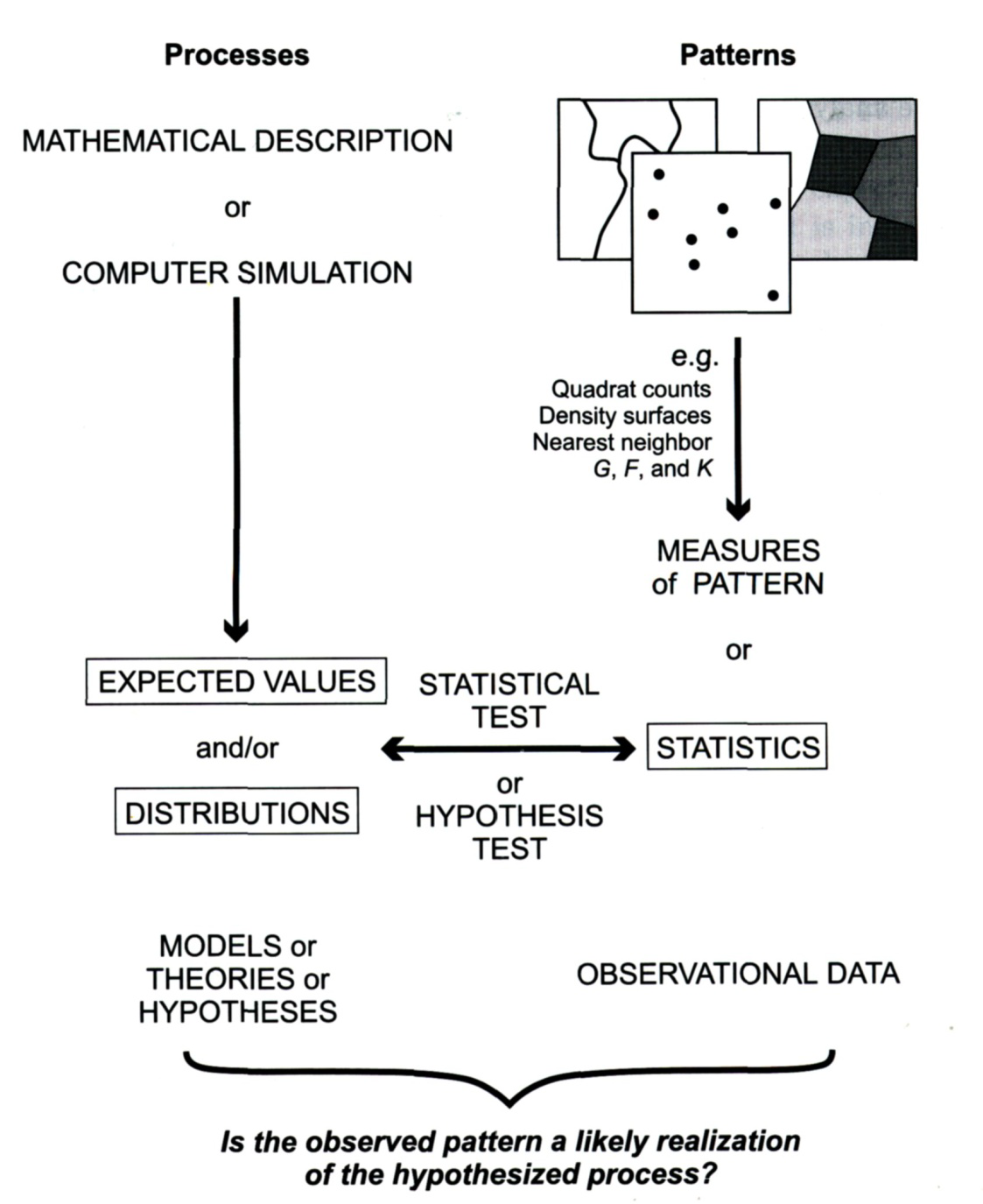
  • A measure describing a point pattern can be predicted for a particular process
  • Many measures for point patterns exist…

Statistical Hypothesis Testing


  • Hypothesis: A statement about the study population that we are interested in determining the truth-value of-we want to assign a likelihood to the hypothesis
  • Null hypothesis (\(H_0\)): what we would see if there were no effect
  • Alternative hypothesis (\(H_1\) / \(H_A\)): This is what we are trying to find evidence to support (not “prove”)

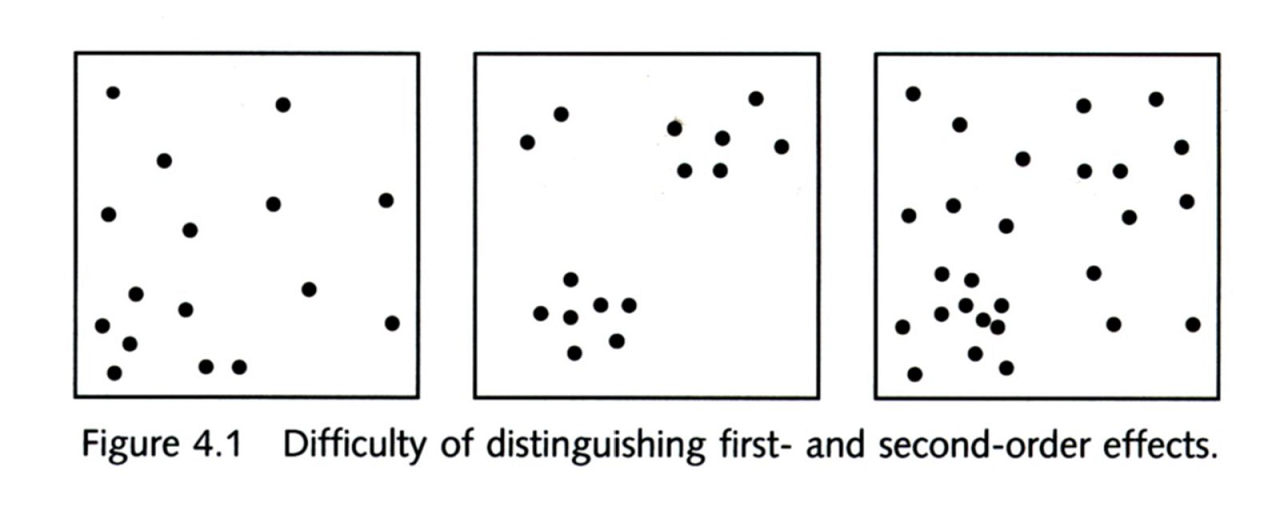
First & Second Order Variation

  • First order variation is characterized by variation in point pattern density or intensity
  • Second order variation is characterized by variation in the distances between events


Some Notation


A point pattern is a set of events, S

$$S = \{S_1,S_2,S_3, ... S_n\}$$

Each event has two coordinates

$$S = (S_{ix}, S_{iy})$$

The study region is represented by A, and it has area a

Centrographic Statistics


  • Single, summary measures of a spatial distribution
  • Mean center of the pattern, \(\bar{S}\) (mean X and Y coordinates)
  • Standard distance, d (how dispersed events are around the mean center)
  • Useful for comparing point patterns or for tracking change over time

U.S. Mean Center of Population

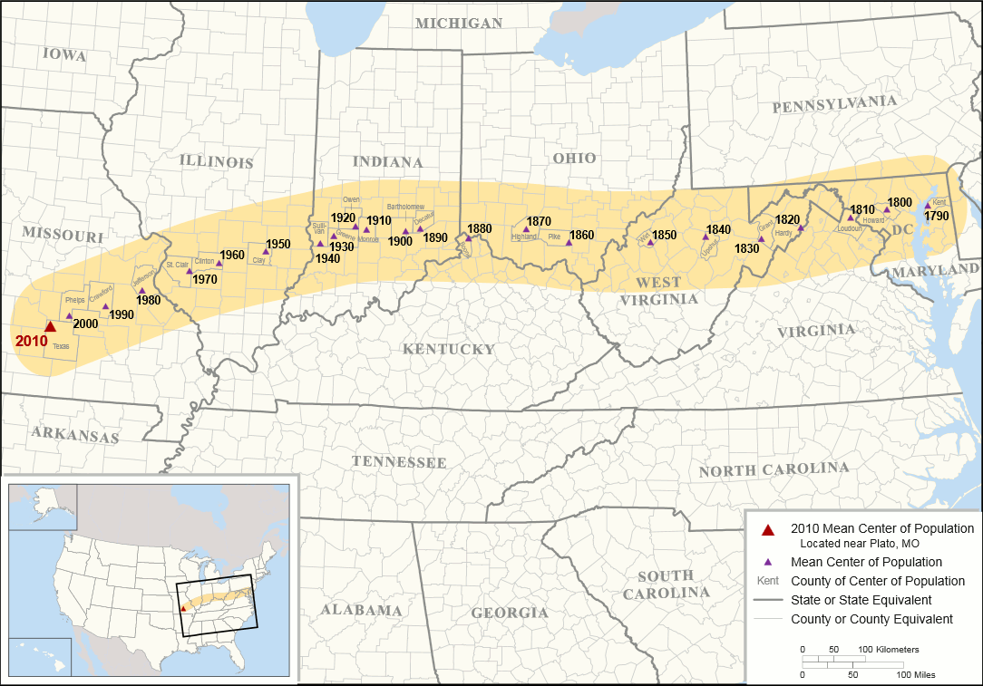
http://maptd.com/2010-united-states-mean-centre-of-population/


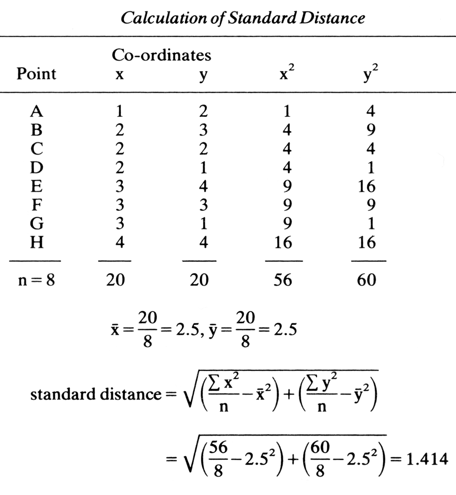
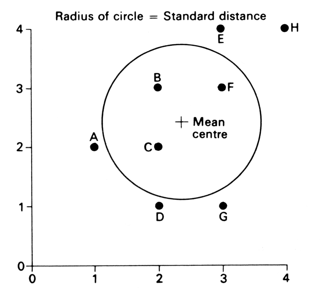
Standard Distance Graph


Describing Poing Patterns - Density-based


Quadrat analysis

Kernel density estimation

Describing Poing Patterns - Distance-based


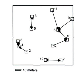
Nearest neighbor analysis

Ripley’s K function

Types of Distribution

Random


Any point is likely to occur at any location, and the position of any point is not affected by the position of any other point.


There is no apparent ordering of the distribution

Uniform


Every point is as far from all of its neighbors as possible

Clustered


Many points are concentrated close together, and there are large areas that contain few (if any) points

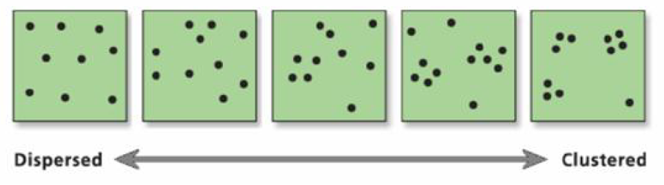
Distribution Examples


Quadrat Anaysis

Quadrat Sampling

Random Placement with Hexagonal Quadrats

Completed Coverage with Regular Quadrats

Quadrat Analysis

  • Based on a measure derived from data obtained after a uniform grid network is drawn over a map of the distribution of interest
  • The frequency count-the number of points occurring within each quadrat-is recorded first
  • These data are then used to calculate variance
  • The variance compares the number of points in each grid cell with the average number of points over all of the cells (variance mean ratio)
  • The variance of the distribution is compared to the characteristics of a random distribution to test the hypothesis

Statistical Mean and Sample Variance


  • Variance-Mean Ratio (VMR) is calculated accross Quadrats:
    • VMR ~= 1: Random
    • VMR < 1: Dispersed
    • VMR > 1: Clustered

Quadrat Analysis Weaknesses


  • Size, shape, and orientation change results
    • Too small: missed patterns
    • Too large: coarse analysis

Same results… different pattern


So what do we do?

An Alternative


  • Nearest Neighbor
  • Higher-ordered neighborhood statistics
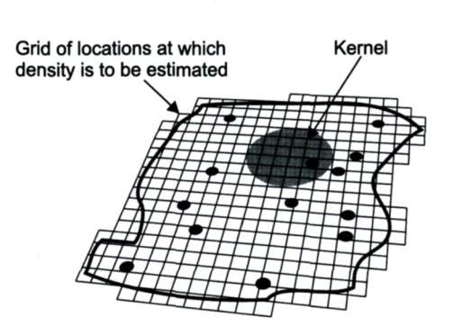
Kernel Density Estimation (KDE)

Kernel Density Estimation (KDE)


  • Nonparametic way of estimating the probability density function of a random variable
  • Data smoothing allows population inference from sample
  • KDE assumes the pattern has a density at any location - what type of data is this? a field!

Kernel Density Estimation (KDE)


Similar to quadrat counting approches:

  • Looks at distances between events in a point pattern
  • Assumes that density is continuously varying and present
  • Centers a circle at a location and counts events within

KDE Example

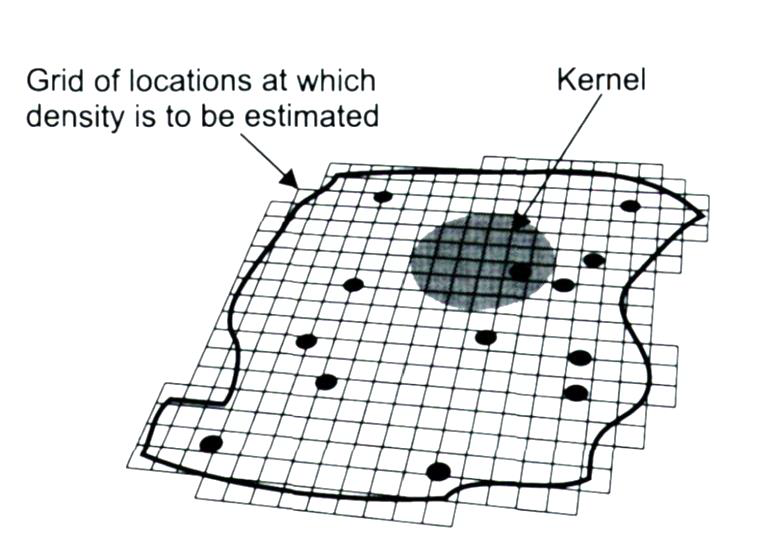
  • place grid over study area
  • calculate density as \(KDE = \frac{n_i}{a_i}\) (where \(n_i\) = count within kernel; \(a_i\) = kernel area)

KDE Example

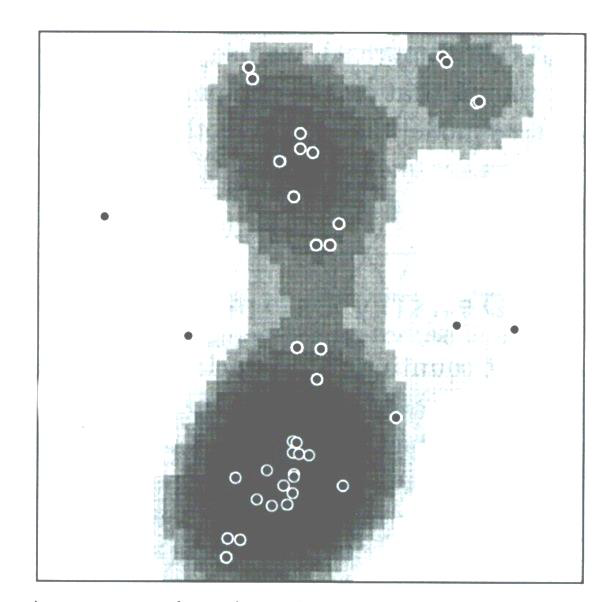
Typical output surface from KDE, and its original point pattern

KDE Example

st_kde <- function(points,cellsize, bandwith, extent = NULL){
  require(MASS)
  require(raster)
  require(sf)
  if(is.null(extent)){extent_vec <- st_bbox(points)[c(1,3,2,4)]} else{extent_vec <-st_bbox(extent)[c(1,3,2,4)]}
  
  n_y <- ceiling((extent_vec[4]-extent_vec[3])/cellsize)
  n_x <- ceiling((extent_vec[2]-extent_vec[1])/cellsize)
  
  extent_vec[2] <- extent_vec[1]+(n_x*cellsize)-cellsize
  extent_vec[4] <- extent_vec[3]+(n_y*cellsize)-cellsize
  
  coords <- st_coordinates(points)
  matrix <- kde2d(coords[,1],coords[,2],h = bandwith,n = c(n_x,n_y),lims = extent_vec)
  raster(matrix)
}
dam_kde <- st_kde(dams %>% filter(State %in% c("Oregon","Washington")),0.1,1)
x <- tmap_leaflet(tm_shape(dam_kde) + 
  tm_raster(title='KDE Estimation',palette = 'Blues', alpha = 0.65) +
  tm_shape(dams %>% filter(State %in% c("Oregon","Washington"))) +
  tm_dots(col='red'))

htmlwidgets::saveWidget(x,"~/documents/teaching/geog597/maps/6_dams_kde.html",selfcontained = T)

Our dams as KDE!